Week 1-1. Numeric and graphic summary
Before we start … let’s install R packages first!
install.packages(c("tidyverse", "gapminder"))library(tidyverse)
library(gapminder)1. Data types

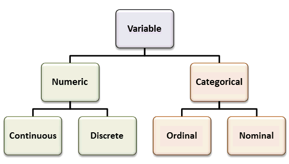
e.g.
- Numeric-Continuous: height, weight, age, etc.
- Numeric-Discrete: number of hospitalization to hospital A
- Categorical-Ordinal: satisfaction score on a scale of 1-not at all happy to 5-very happy
- Categorical-Nominal: 1-male/0-female, 1-smoker/0-non-smoker
2. Histogram

- A
histogramplots the distribution of a numeric variable’s values using bars - Cannot plot a histogram with a categorical variable!
- Histogram is about only one single variable. Histogram does not show the relationship of two variables.
- Each bar represents a range of numeric values called “bin” or “class”
- A bar’s height = frequency of data points with a value within the corresponding bin.
[R code]
# Load the 'gapminder' dataset
df <- gapminder

# Print first 6 rows
head(df)
## # A tibble: 6 × 6
## country continent year lifeExp pop gdpPercap
## <fct> <fct> <int> <dbl> <int> <dbl>
## 1 Afghanistan Asia 1952 28.8 8425333 779.
## 2 Afghanistan Asia 1957 30.3 9240934 821.
## 3 Afghanistan Asia 1962 32.0 10267083 853.
## 4 Afghanistan Asia 1967 34.0 11537966 836.
## 5 Afghanistan Asia 1972 36.1 13079460 740.
## 6 Afghanistan Asia 1977 38.4 14880372 786.# Plot a histogram of life expectancy
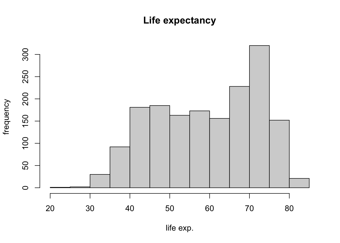
hist(df$lifeExp,
main = "Life expectancy", # plot title,
xlab = "life exp.", # x-axis label
ylab = "frequency", # y-axis label
breaks = "FD" # number of bins
)
- For more methods on how to determine the number of bins, please click HERE.
3. Multiple histograms in one screen
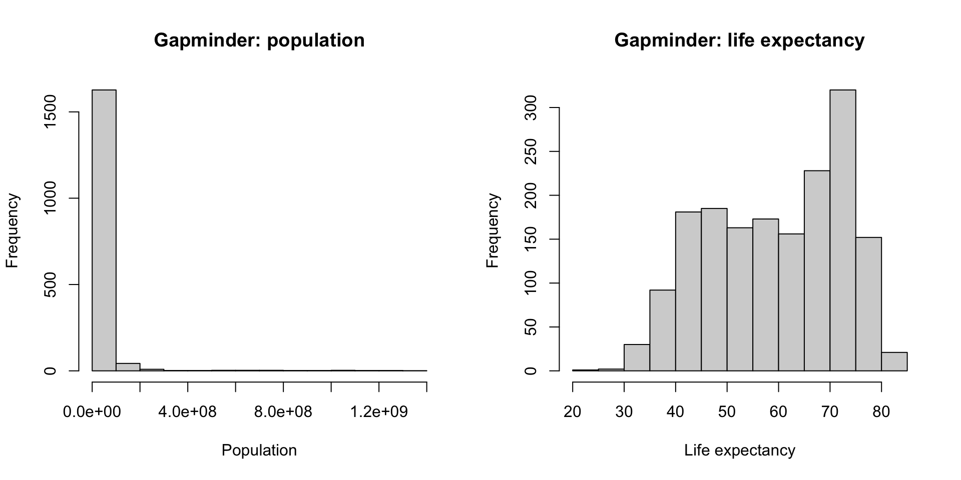
par(mfrow = c(1, 2)): makes side-by-side plots- Here,
c(1, 2)indicates the number of rows and columns.
par(mfrow = c(1, 2))
hist(df$pop, main = "Gapminder: population", xlab = "Population")
hist(df$lifeExp, main = "Gapminder: life expectancy", xlab = "Life expectancy")
4. Summary statistics
- mean:
mean() - median:
median() - standard deviation:
sd() - variance:
var() - quantile:
quantile() - minimum:
min() - maximum:
max() summary()can show these numeric summaries at once
mean(df$lifeExp)## [1] 59.47444median(df$lifeExp)## [1] 60.7125sd(df$lifeExp)## [1] 12.91711var(df$lifeExp)## [1] 166.8517quantile(df$lifeExp)## 0% 25% 50% 75% 100%
## 23.5990 48.1980 60.7125 70.8455 82.6030min(df$lifeExp)## [1] 23.599max(df$lifeExp)## [1] 82.603summary(df$lifeExp)## Min. 1st Qu. Median Mean 3rd Qu. Max.
## 23.60 48.20 60.71 59.47 70.85 82.60