1. Statistical Inference
the process of learning some properties of the population starting from a sample drawn from this population.
For example, you may be in interested in learning about the cholesterol level of patient with heart disease, but we cannot measure the whole population.
But you can measure the cholesterol level of a random sample of the population and then infer or generalize the results to the entire population.
Terms we need to clarify:
- Data generating distribution: the unknown probability distribution that generates the data.
- Empirical distribution: the observable distribution of the data in the sample.
- Parameter: unknown object of interest
- Estimator: data-driven guess at the value of the parameter.
Usually we are interested in a function of the data generating distribution. This is often referred to as parameter (or the parameter of interest)
Use sample in order to estimate the parameter of interest
Use a function of empriical distribution, referred to as estimator.
(Mathematical notation) for parameters, Greek letters, while for estimate, Roman letter.
(Mathematical notation) “hat” notation places a “hat” over the Greek letter for the parameter.
- e.g. \(\hat{\theta}\) is the estimator of the parameter \(\theta\).
- e.g. \(\hat{\theta}_n\) is used when you specifically want to emphasize that we are using a sample of \(n\) observations to estimate the parameter.
2. Example: Cholesterol values in patients with heart disease
Let’s assume that we want to estimate the average cholesterol value of healthy individuals in the United States. Let’s assume that we have cholesterol measurements for a random sample of the population (more on this later!).
- Parameter of Interest: the mean cholesterol value of heart patients in the population, denoted as \(\mu\)
- How can we estimate the parameter using the data in our
sample?
- We would estimate the population mean cholesterol level \(\mu\) with the mean (or average) cholesterol values computed from our sample, denoted by \(\hat{\mu}\) or \(\bar{x}\).
3. More on the data generating distribution
The data generating distribution is unknown when we collect a sample from a population. In non-parametric statistics we aim at estimating this distribution from the empirical distribution of the sample, without making any assumptions on the shape of the distribution for the population values. However, it is often easier to make some assumptions about the data generating distribution. These assumptions are sometimes based on domain knowledge or on mathematical convenience.
One commonly used strategy is to assume a family of distributions for the data generating distribution, for instance the Gaussian distribution or normal distribution.
4. Random Variables and Probability Distributions
1) Probability
In order to make inference from a random sample to the whole population, we need some notion of randomness. To study randomness we need the concept of probability. Hence, probability is one of the foundations of statistical inference.
- What is a probability measure?
- Long story short, our main interest is a probability as a measure
that quntifies the randomness of an event
- e.g. the probability of obtaining ‘heads’ when tossing a coin.
- Long story short, our main interest is a probability as a measure
that quntifies the randomness of an event
- Principles
- The probability of an event is a number between 0 and 1.
- The sum of the probabilities of all possible events is 1.
- The probability of the union of two disjoint events is the sum of their probabilities.
- The probability of two independent events occurring is the product of their probabilities.
2) Random variables
Recall that a variable is a measurement that describe a characteristic of a set of observations. A random variable (r.v.) is a variable that measures an intrinsically random process, e.g. a coin toss. Before observing the outcome, we will not know with certainty whether the toss will yield “heads” or “tails”, but that does not mean that we do not know anything about the process: we know that on average it will be heads half of the times and tails the other half. If we refer to \(X\) as the process of measuring the outcome of a coin toss, we say that \(X\) is a random variable.
- Random variables and statistical inference
- For instance, let’s say that we want to describe the height of a certain population. The height of an individual is not a random quantity! We can measure with a certain amount of precision the height of any individual.
- What is random is the process of sampling a set of
individuals from the population?
- The randomness is the particular set of individuals (and their heights) that we get from the population. The height of a known individual in our sample is not random. Rather the fact that this particular individual is in our sample is random. Hence, the individuals that compose our particular sample is random. If two researchers each took a random sample of 100 adults from the population, they each would have a different set of individuals (with maybe a few people being in both sets).
- the randomness comes from the sampling mechanism, not from the quantity that we are measuring: if we repeat the experiment, we will select a different sample and we will obtain a different set of measurements.
- Continuous and discrete random variables
- A discrete random variable can only take a countable number of possible outcomes (e.g., a coin flip, or the number of operations a patient has had).
- A continuous random variable can take any real value. An example of a continuous random variable is the weight of a participant in a clinical trial.
5. Probability distributions
- 4 key quantities:
- Probability Mass Function (PMF) for discrete / Probability Density Function (PDF) for continuous
- Cumulative Distribution Function (CDF)
- Quantiles
- Expected Value
6. Probability Mass Function (PMF)
\(S\): Sample space or the space of all the possible values of \(X\)
The PMF of a discrete random variable \(X\) is a function \(p\) with the follwing properties.
- Non-negativity
\[ p(x)>=0 \quad \forall x) \in S \]
- Sum across all values is one
\[ \sum_{x \in S} p(x)=1 \]
- Example: Number of heads in 10 coin flips
set.seed(1)
rbinom(n = 1, size = 10, prob = 0.5)
## [1] 4- If we repeat the experiment,
rbinom(n = 1, size = 10, prob = 0.5)## [1] 4- Different result
- Now we could ask, if we flip a coin 10 times, what is the probability
of getting 0 heads? 1 heads? 2 heads, . . . 10 heads?
- Since this is all the possibilities, this set of probabilities is the PMF.
- What is the the PMF, e.g. what is the probability distribution of
flipping a coin 10 times?
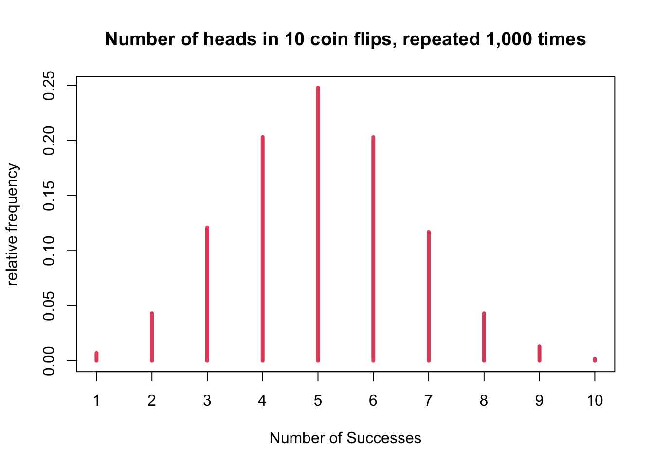
- One way to answer is by repeating the experiment many, many times, say 1,000. We can have R repeat this experiment for us rather than us doing this tedious work.
(x <- rbinom(n = 1000, size = 10, prob = 0.5))## [1] 5 7 4 7 7 6 6 3 4 4 6 5 6 5 6 9 5 6 7 4 6 3 4 5
## [25] 2 5 7 4 5 5 5 4 6 6 6 3 6 5 6 6 6 5 5 6 2 5 6 6
## [49] 5 7 5 4 3 3 4 5 6 5 7 4 5 4 6 4 5 6 3 7 4 7 4 4
## [73] 5 7 7 5 6 8 5 6 5 4 6 4 6 3 4 3 4 3 6 7 6 6 5 5
## [97] 6 5 6 4 4 9 6 4 3 5 7 5 8 6 4 5 3 2 6 3 5 6 9 5
## [121] 5 4 6 5 5 4 4 5 5 3 2 6 7 5 5 5 8 5 6 5 4 4 6 5
## [145] 4 6 3 7 5 5 4 5 5 4 5 3 4 4 4 7 5 6 7 5 3 4 6 4
## [169] 6 7 7 5 5 7 6 6 5 7 4 4 7 5 7 4 6 6 7 5 6 5 3 7
## [193] 4 5 3 7 4 6 4 4 5 4 4 5 5 3 4 6 8 3 6 8 6 4 6 8
## [217] 8 4 4 3 4 5 7 5 4 2 5 7 4 3 4 6 5 6 6 5 5 5 4 5
## [241] 7 3 5 4 5 3 5 7 6 7 5 5 5 3 4 5 4 7 5 4 4 6 6 3
## [265] 3 6 5 3 3 3 5 3 4 4 4 4 5 6 2 5 7 4 2 3 4 3 3 4
## [289] 4 3 8 4 5 6 3 3 2 7 6 3 5 5 4 9 4 6 3 5 3 4 7 6
## [313] 4 5 3 4 8 6 6 4 5 9 7 8 6 6 4 6 8 4 5 6 3 4 5 3
## [337] 5 8 9 4 5 5 6 4 5 3 4 6 5 3 6 5 8 4 7 3 7 5 3 4
## [361] 7 4 5 7 3 6 6 5 5 5 7 4 4 5 4 7 4 5 5 5 6 8 4 4
## [385] 6 7 3 8 3 3 7 5 3 4 6 4 4 3 6 4 8 7 7 6 4 6 2 7
## [409] 9 4 6 6 6 5 5 4 6 6 5 5 6 3 4 5 3 7 7 7 7 3 5 5
## [433] 3 6 6 2 5 7 2 4 5 5 4 5 4 7 3 3 8 5 4 3 2 6 5 8
## [457] 5 3 3 5 1 5 4 7 6 3 5 6 5 8 6 5 3 4 7 5 5 6 6 3
## [481] 7 8 5 5 4 1 7 3 2 7 4 3 5 5 5 5 7 3 5 6 6 6 5 8
## [505] 5 7 6 5 7 5 1 6 6 4 6 5 4 6 7 6 4 3 5 7 6 6 8 9
## [529] 5 2 4 4 3 2 4 4 4 5 5 8 6 4 4 3 9 5 5 6 7 5 2 7
## [553] 6 5 3 2 6 7 6 3 4 6 7 6 4 6 4 8 3 5 4 3 6 5 6 5
## [577] 7 6 4 8 6 2 5 5 3 5 8 6 5 4 6 6 7 6 5 5 5 5 6 7
## [601] 3 6 8 8 4 5 8 3 7 4 5 5 6 5 3 4 6 3 7 4 5 3 4 5
## [625] 4 6 5 7 7 4 4 7 5 4 3 3 6 6 7 4 7 4 6 4 2 7 6 7
## [649] 6 7 4 5 5 3 4 5 6 7 4 6 3 6 4 5 7 4 4 6 6 5 6 5
## [673] 5 5 4 3 4 4 6 6 3 5 5 5 5 5 2 7 3 5 6 5 5 5 6 3
## [697] 8 5 7 7 6 6 6 3 5 5 7 6 6 5 3 6 5 5 2 3 5 6 1 5
## [721] 7 6 4 7 4 5 5 2 6 5 6 2 6 4 4 7 3 2 4 5 5 4 4 5
## [745] 5 7 3 6 5 7 5 3 5 4 5 4 8 5 6 3 7 4 4 3 5 6 7 6
## [769] 5 6 2 9 6 5 2 6 4 10 7 6 6 5 7 3 5 4 5 2 4 3 7 4
## [793] 5 6 4 5 6 4 7 2 8 6 4 6 4 8 4 2 4 5 4 8 5 5 7 7
## [817] 4 6 4 5 6 6 7 2 4 4 4 6 6 7 7 6 5 5 3 7 8 5 7 3
## [841] 4 5 5 5 2 6 6 4 8 6 2 8 4 2 4 6 4 4 2 4 6 2 3 5
## [865] 5 6 6 3 5 8 6 4 5 2 4 5 6 9 4 7 8 7 5 6 6 6 5 4
## [889] 1 3 3 2 4 3 5 2 1 3 7 6 4 4 4 3 3 3 3 2 5 6 6 3
## [913] 2 5 3 6 6 7 4 8 8 2 7 6 6 4 5 5 5 7 4 4 6 6 7 5
## [937] 7 4 4 7 2 5 5 5 6 6 7 6 3 4 6 7 5 4 7 4 5 1 4 5
## [961] 3 6 4 4 4 7 9 6 9 5 5 8 3 3 2 5 6 6 3 3 8 5 4 5
## [985] 5 4 10 5 3 5 5 4 3 6 6 4 4 4 5 6- x: the number of times we got 0, 1, 2, 3, …, 10 head out of 10 flips of a fair coin in 1000 experiments.
- Plot the probability distribution based on 1000 experiments
plot(table(x) / sum(table(x)), type = 'h', col = 2, lwd = 4,
    xlab = "Number of Successes",
    ylab = "relative frequency",
    main = "Number of heads in 10 coin flips, repeated 1,000 times")
7. Example of PMF: Binomial Distribution
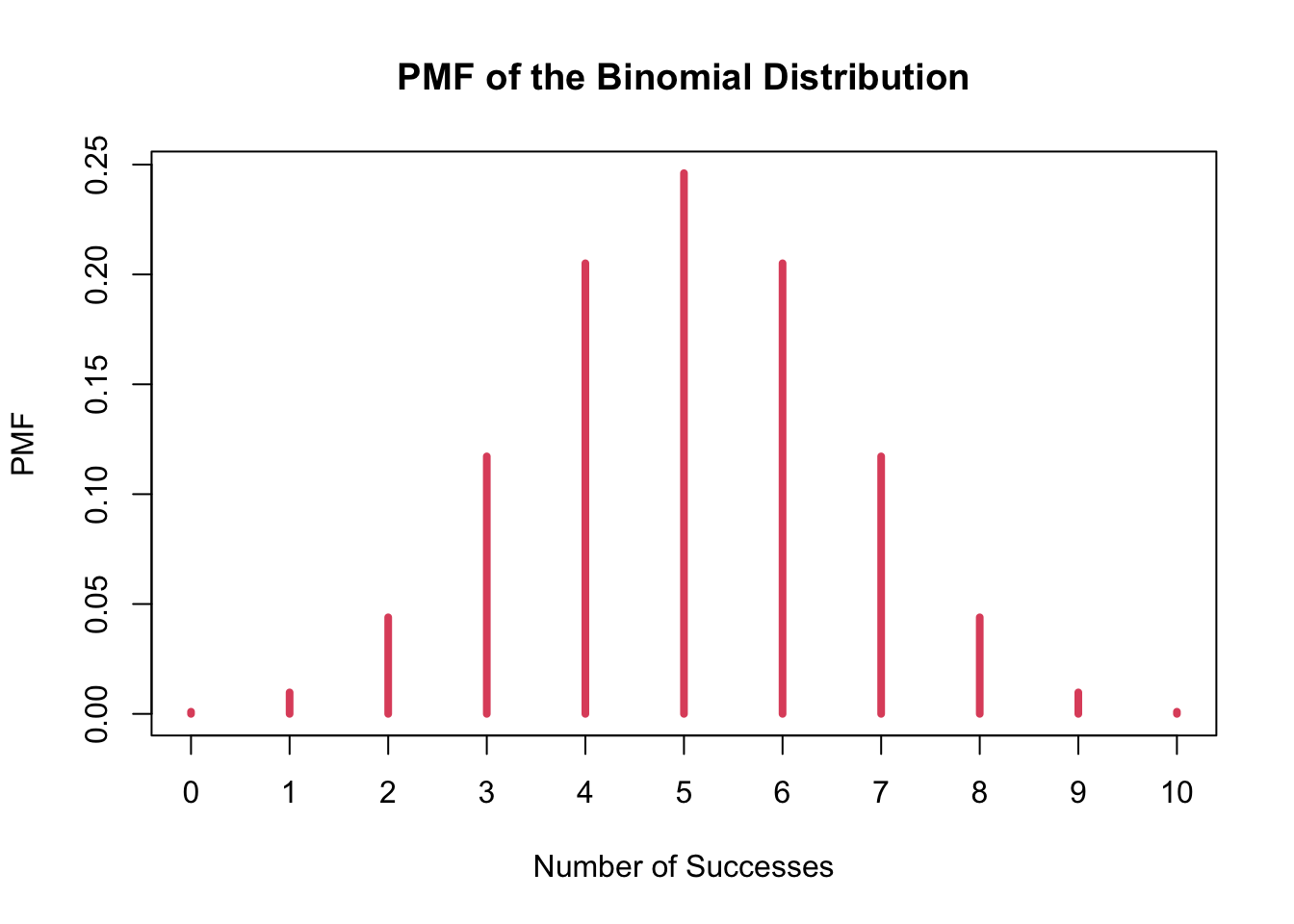
- There is also a mathematical formula that describes the PMF for the number of heads when flipping a fair coin 10 times. It is called the binomial distribution.
- PMF of the number of successes out of \(n\)tries where a probability of success is \(\pi\) is
1) dbinom() function -1
dbinom()function can be used to compute the binomial PMF.x: the number of “successes”, which in this case is the number of heads.- size: the number of “tries”, which in this case 10 flips
- prob: the probability of getting a success in a single try, which in this case is the probability of getting a head in one flip, 0.5.
dbinom(x = 5, size = 10, prob = 0.5)## [1] 0.24609382) dbinom() function -2
dbinom()also can be used to show the entire distribution by setting up x as a vector.- If we have 10 tries (flips), then the set of the possible number of successes (heads) is x = 0, 1, 2, . . . , 10. We will save the probabilities in a variable ‘p’.
(p <- dbinom(x = 0:10, size = 10, prob = 0.5))## [1] 0.0009765625 0.0097656250 0.0439453125 0.1171875000 0.2050781250
## [6] 0.2460937500 0.2050781250 0.1171875000 0.0439453125 0.0097656250
## [11] 0.00097656253) plotting the binomial distribution’s PMF
- x-axis: the possible values of the random variable
- y-axis: the probability of observing that value
pmf <- as.table(p)
names(pmf) <- 0:10
plot(pmf, col = 2, lwd = 4,
    xlab = "Number of Successes",
    ylab = "PMF",
    main = "PMF of the Binomial Distribution")
4) Accuracy of the simulation
- We can verify that our simulation was actually quite accurate.
- Specifically, recall that we used
rbinom()function to simulate performing the experiment of 10 coin flips 1000 times and for each experiment of 10 flips, we recorded the number of heads. - Let’s compare how our computed distribution for the probability of each outcome compares to the exact probability obtained from the mathematical formula for the binomial PMF.
- Specifically, recall that we used
table(x) / sum(table(x))## x
## 1 2 3 4 5 6 7 8 9 10
## 0.007 0.043 0.121 0.203 0.248 0.203 0.117 0.043 0.013 0.002round(pmf, 3)## 0 1 2 3 4 5 6 7 8 9 10
## 0.001 0.010 0.044 0.117 0.205 0.246 0.205 0.117 0.044 0.010 0.0018. Probability Density Function (PDF) (i.e., density function)
- The analog of the PMF for continuous distributions is the probability density function, or simply density function.
- The properties of the PDF are similar to those of the PMF, but
extended to the case of real numbers.
- Non-negativity:
\[ p(x)>=0 \quad \forall x) \in S \]
- The total area under the curve is 1:
\[ \int_{x \in S} f(x)=1 \]
- Areas under the PDF represent probabilities.
- In particular, the probability of an individual value.
- Say \(x\) is 0. However, the probability of \(x-\delta x \text { to } x+\delta x\) is a number greater than 0 for any \(\delta\), no matter how small.
9. Example of PDF: Gaussian (Normal) Distribution
- To denote a particular normal distribution, you need to specify its mean and its variance.
- A standard normal is a normal random variable with mean zero and variance of one.
\[ f(x)=\frac{1}{\sqrt{2 \pi \sigma^{2}}} e^{-\frac{(x-\mu)^{2}}{2 \sigma^{2}}}, \text { where }-\infty<x<\infty \]
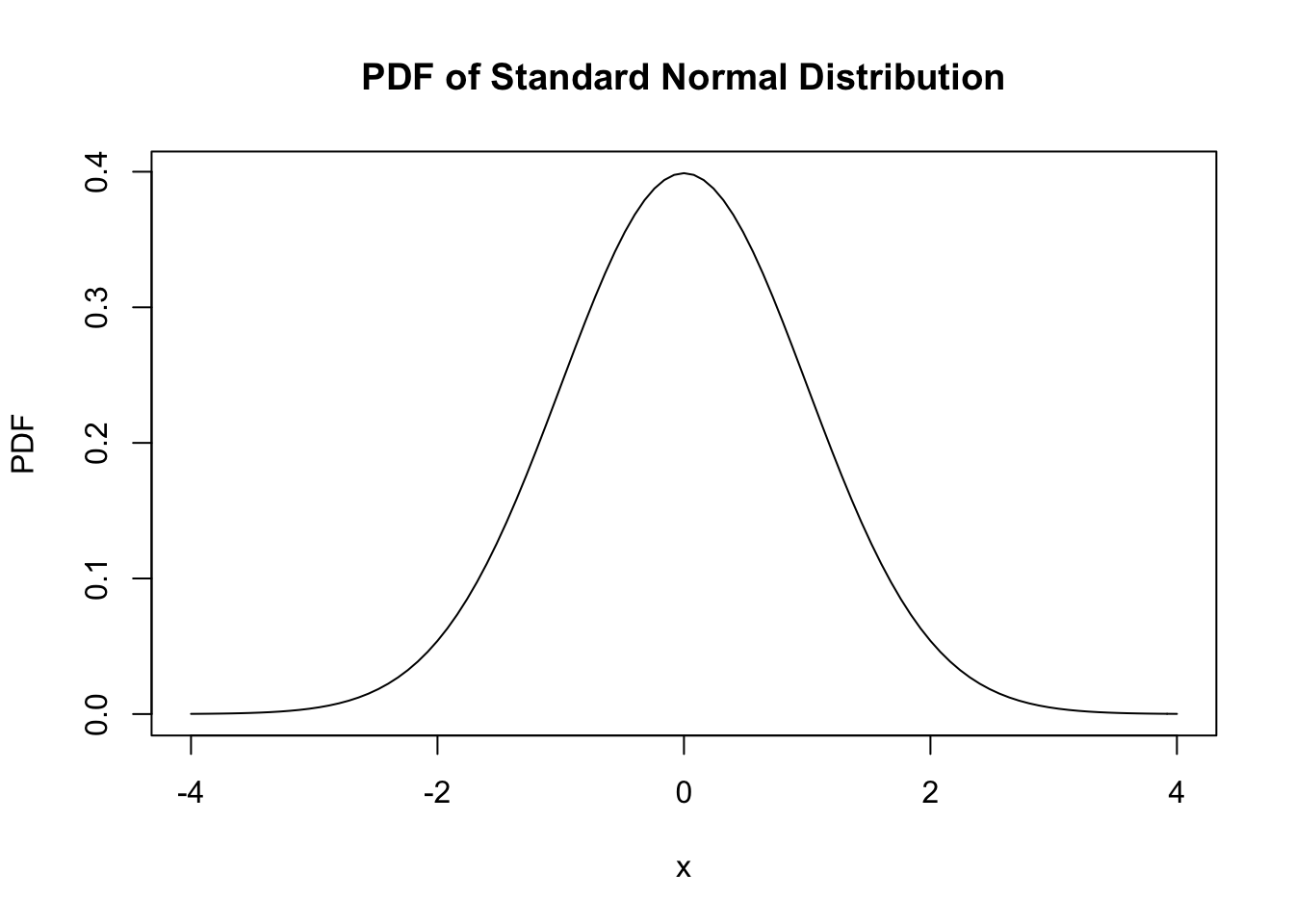
- Plotting the normal distribution
curve(dnorm, from = -4, to = 4,
     xlab = 'x',
     ylab = "PDF",
     main = "PDF of Standard Normal Distribution")
- Just like
dbinom(), we can usednorm()function to get the value of the density for any real number. - However, this is NOT the probability of getting
that value
dnorm(1)gives thef(1), which is the value from the curve for a standard normal distribution (since specific values for the mean and standard deviation were note specified) and it is NOT the probability of getting a 1 from a standard normal distribution.- Instead, this probability would be 0 (zero).
- (NOTE) PDF does not give you the probability of the event!
- Since continuous variables can take infinite number of values, the probability of any specific value is 0. (otherwise the sum under the curve would be greater than 1).
- Thus, we always make statements on the probabilities of
intervals.
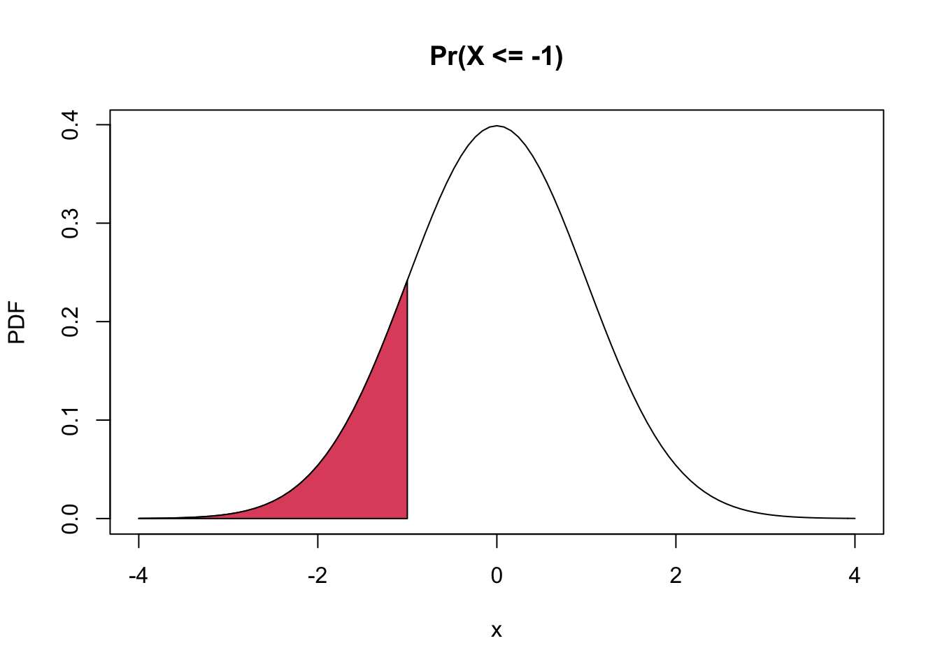
- e.g. if X is a standard normal random variable, what is the probability that X is less than -1?
curve(dnorm, from = -4, to = 4,
     ylab = 'PDF',
     main = 'Pr(X <= -1)')
coord.x <- c(-4, seq(-4, -1, by = 0.1), -1)
coord.y <- c(0, dnorm(seq(-4, -1, by = 0.1)), 0)
polygon(coord.x, coord.y, col = 2)
10. Cumulative Distribution Function (CDF)
- One important quantity linked to the area under the PDF is the cumulative distribution function.
- the probability that a random variable is less or equal than a certain number.
\[ F(x)=\operatorname{Pr}(X \leq x) \]
- Both applies to continuous and
discrete random variables.
- Relationship between PDF-CDF:
\[ F(x)=\int_{X \leq x} f(x) d x \]
- Relationship between PMF-CDF:
\[ F(x)=\sum_{X \leq x} p(x) d x \]
Example: Gaussian (Normal) Distribution
pnorm(): to compute the CDF of the normal distribution variable, or to compute the probability of any interval.- e.g. the probability that \(X\) is less than -1 is
pnorm(-1, 0, 1)## [1] 0.1586553- e.g. Pr(X>2)=1-Pr(X<=2)=1-F(2)
1 - pnorm(2)## [1] 0.02275013- e.g. the probability that \(X\) is between -1 and 1
- i.e., Pr(-1<=X<=1)=Pr(X<=1) - Pr(X<=-1) = F(1) - F(-1)
pnorm(1) - pnorm(-1)## [1] 0.682689511. Quantiles
- the \(p\) quantile is the number \(q\) such that \(p\) X 100% of the observations are less than or equal to \(q\).
\[ F(q)=\operatorname{Pr}(X \leq q)=p \]
- Note that we are interested in the quantile \(q\), after fixing the probability \(p\), therefore
\[ q=F^{-1}(p) \]
Example: Gaussian (Normal) Distribution
qnorm(): to compute the quantiles of the standard normal distribution.- e.g. 0.95-quantile for a standard normal
qnorm(0.95) # equal to qnorm(0.95, 0, 1)## [1] 1.64485412. Summary: PDF, CDF, and quantiles in R
dnorm(): to compute the PDF of a normal random variablepnorm(): to compute its CDFqnorm(): to compute is quantile.rnorm(): to generate (siulate) a random sample from the normal distribution
13. Expected Value and Variance
1) Expected Value
The expected value or mean of a random variable is the center of its distribution.
In case \(X\) is a discrete random variable, the expected value is
\[ E[X]=\sum_{x \in S} x p(x) \]
where p(x) is the PMF of X.
- In case \(X\) is a continuous random variable, the expected value is
\[ E[X]=\int_{x \in S} x f(x) d x \]
where f(x) is the PDF of X.
2) Expected Value and Sample Mean
- Sample mean is what we will use to estimate the expected value, or the mean of the data generating distribution.
- Sample mean: the mean of the empricial distribution of the sample, which is obtained by giving probability 1/n to each observed value.
\[ p_{n}(x)=\sum_{i=1}^{n} x_{i} p_{n}\left(x_{i}\right)=\frac{1}{n} \sum_{i=1}^{n} x_{i} \]
3) Variance
- Variance of a random variable is the following way.
- In case of the \(\mu\), the epected value of \(X\), the variance is
\[ \operatorname{Var}(X)=E\left[(X-\mu)^{2}\right] \]
\[ \operatorname{Var}(X)=E\left[X^{2}\right]-E[X]^{2} \]
4) Sample Variance
- Formula
\[ S^{2}=\frac{1}{n-1} \sum_{i=1}^{n}\left(x_{i}-\bar{x}\right)^{2} \]
where \(\bar{x}\) is sample mean.
- As the variance is the mean of the squared differences from the expected value, the sample variance is (almost) the mean of the squared differences from the sample mean.
14. Parameters of a distribution
- binomial distribution
- \(n\): the number of trials
- \(\pi\): the probability of success
- normal distribution
- \(\mu\): the expected value or the mean
- \(\sigma\): standard deviation