1. Review binomial random variable
- If \(Y\) = number of success in
\(n\) independent trials, then \(Y\) is a binomial random
variable with \(\pi\) =
probability of success.
- \(Y~B(n, \pi)\)
- PMF of \(Y\):
\[ p_{Y}(y)=\sum_{n=0}^{n}\left(\begin{array}{l}n \\ k\end{array}\right) \pi(1-\pi) \quad y=0,1, \ldots, n \]
- Expected value of \(Y\), \(E(Y)\) is determined by
\[ p_{Y}(y)=\sum_{n=0}^{n} y \times\left(\begin{array}{l}n \\ k\end{array}\right) \pi(1-\pi)=n \pi \]
2. Sample Proportion
- The sample proportion is a random variable and can be defined as:
\[ E(P)=E\left(\frac{Y}{n}\right)=\frac{E(Y)}{n}=\frac{n \pi}{n}=\pi \]
- This is an example of the method of moments.
Method of Moments
a way of estimating parameters, based on matching a moment of the data-generating distribution with the related moment of the empirical distribution
2.1 The Maximum Likelihood Estimator (MLE)
- Maximum likelihood estimator (MLE) is the quantity that maximizes the likelihood function.
2.2 The Likelihood Function
- The likelihood function is the probability mass
function (PMF) or density (PDF) evaluated at the data \(X_1,...,X_n\), views as a function
of the parameter.
- Assume we have a set of discrete independent and identically distributed (i.i.d.) random variable’s, \(X_1,...,X_n\) whose distribution depends on a parameter \(\theta\).
- Denote the PMF of each \(X_i\) as \(p(x \mid \theta)\)
- the likelihood is then
\[ L(\theta)=\prod_{i=1}^{n} p\left(x_{i} \mid \theta\right) \]
- But it is often more useful to compute the log-likelihood function:
\[ l(\theta)=\sum_{i=1}^{n} \log p\left(x_{i} \mid \theta\right) \]
- View the above as a function of the parameter.
- Thus, it is important to define the parameter space or the set of values that a parameter can take.
2.3 Example: Likelihood of a Binomial Sample
Suppose that we want to test whether a coin is fair, i.e., if the probabilities that it lands on “heads” or “tails” are the same. We can flip the coin a few times, say \(n=15\) and see how many times it give “heads” (\(x=1\)) or “tails” (\(x=0\)). Then \(Y=X_1+...+X_n\) is a **binomial random variable, \(Y~B(n, \pi)\).
- More formally, we have a series of i.i.d. Bernoulli random variables (which you can think of as a Binomial with \(n=1\)), \(X_1,...,X_n\), such that
\[ X_{i} \sim B(1, \pi) \]
- We don’t know \(\pi\) since we
don’t know whether the coin is fair, but we know the observed
values of x_i in that we performed the experiment.
- We can compute the **likelihood function of the \(n\) Bernoulli trials:
\[ L(\pi)=\prod_{i=1}^{n} \pi^{x_{i}}(1-\pi)^{1-x_{i}}, \quad x_{i} \in\{0,1\} \]
- And the log-likelihood function is
\[ \begin{aligned} l(\pi) &=\sum_{i=1}^{n} x_{i} \log \pi+\left(1-x_{i}\right) \log (1-\pi) \\ &=n {\log }(1-\pi)+(\log \pi-\log (1-\pi)) \sum_{i=1}^{n} x_{i} \end{aligned} \]
R
set.seed(1)
(x <- rbinom(15, size = 1, prob = .5))
## [1] 0 0 1 1 0 1 1 1 1 0 0 0 1 0 1loglik <- function(pi, data) {
sum(log(dbinom(data, size = 1, prob = pi)))
}
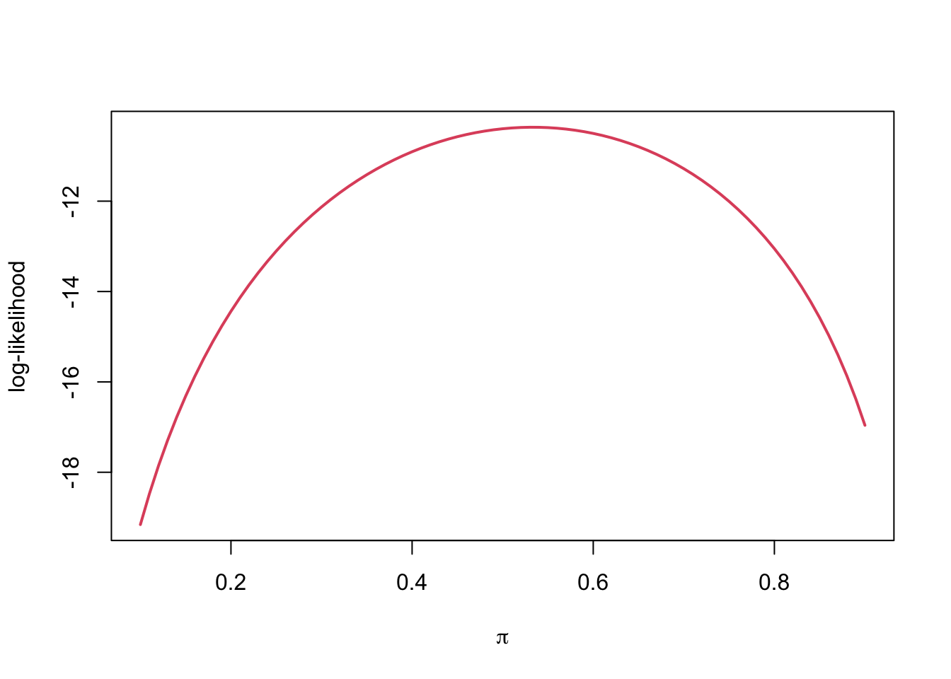
loglik(pi = .5, data = x) %>% round(3)## [1] -10.397loglik(pi = .4, data = x) %>% round(3)## [1] -10.906- Plot the likelihood over a range of \(\pi\) values
pis <- seq(0.1, 0.9, by = 0.01)
ll <- sapply(pis, loglik, data = x)
plot(pis, ll, type = 'l', col = 2, lwd = 2,
     xlab = expression(pi),
     ylab = 'log-likelihood')
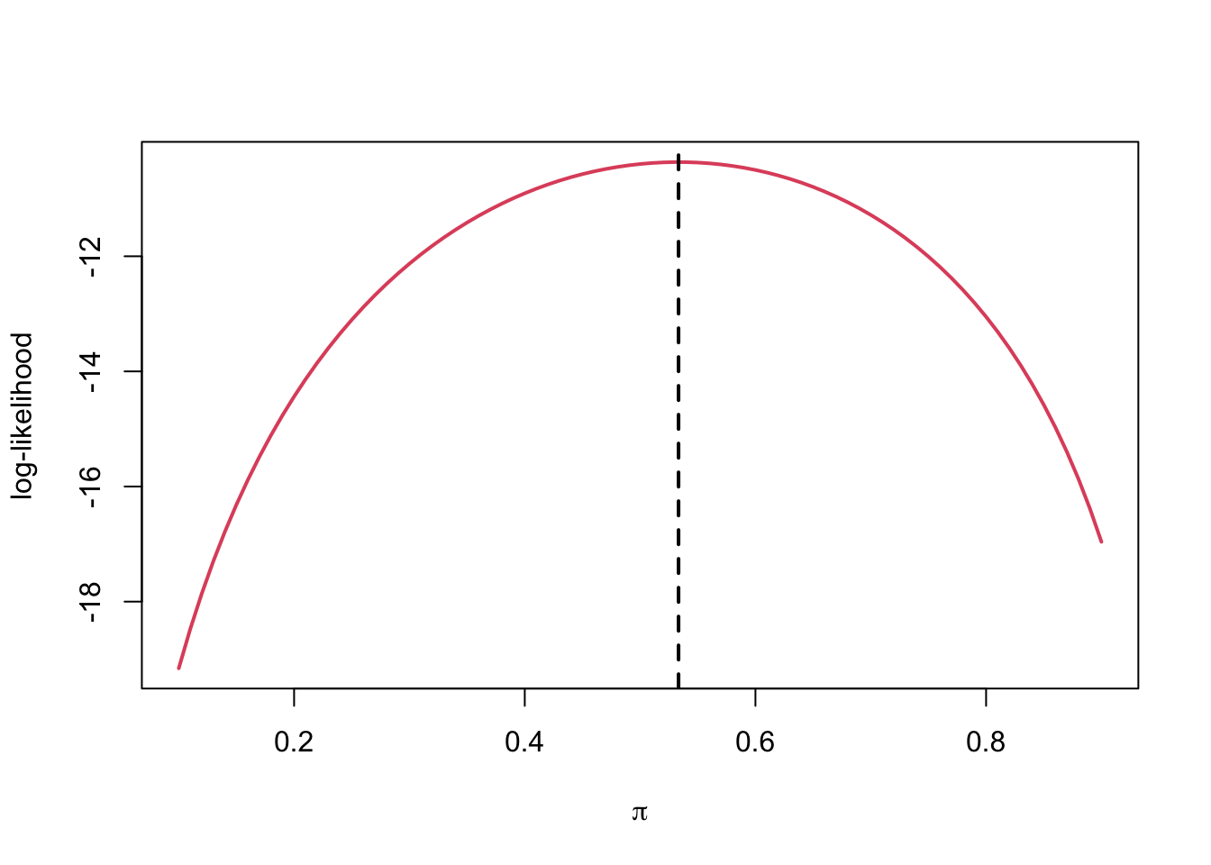
- The maximum likelihood estimator (MLE) is the
parameter value that maximizes the likelihood (or log-likelihood)
function.
- Take the derivative of the log-likelihood function with respect to the parameter, \(\theta\).
- Find the value of the parameter for which the derivative = 0.
\[ \begin{aligned} \frac{d l(\pi)}{d \pi}=& \frac{1}{\pi(1-\pi)} \sum_{i=1}^{n} x_{i}-\frac{n}{1-\pi} \\=& \frac{\sum_{i=1}^{n} x_{i}-n \pi}{\pi(1-\pi)} \\=& 0 \\ & \hat{\pi}=\frac{1}{n} \sum_{i=1}^{n} x_{i} \end{aligned} \]
R
plot(pis, ll, type = 'l', col = 2, lwd = 2,
     xlab = expression(pi),
     ylab = 'log-likelihood')
abline(v = mean(x), lty = 2, lwd = 2)
3. Properties of the estimators
3.1 Properties of estimators: Bias
- An estimator, \(\hat{\theta}\), is a random variable for which we can compute mean and variance.
- Can define the bias of an estimator as:
\[ \operatorname{Bias}=E[\hat{\theta}]-\theta \]
- An unbiased estimator is when
\[ E[\hat{\theta}]=\theta \]
3.2 Mean Squared Error (MSE)
- When we compare two estimators, we care both bias and variance.
- We may prefer a biased estimator over an unbiased one, if the bias estimator has smaller variance.
- Bias-variance tradeoff
- A measure to compare two estimators is the mean squared error (MSE), which combines bias and variance.
\[ M S E[\hat{\theta}]=E\left[(\hat{\theta}-\theta)^{2}\right]=\operatorname{Var}(\hat{\theta})+\operatorname{Bias}(\hat{\theta})^{2} \]
3.3 Consistency
- An estimator, \(\hat{\theta}\), is
consistent, as \(n\)
goes to infinity, it converges in probability to the true parameter
value \(\theta\). For any \(\varepsilon>0\).
- There are two methods.
\[ \begin{array}{c}1) \lim _{n \rightarrow \infty} \operatorname{Pr}\left(\left|\hat{\theta}_{n}-\theta\right|>\varepsilon\right)=0 \\ 2) \lim _{n \rightarrow \infty} M S E\left(\hat{\theta}_{n}\right)=0\end{array} \]
3.4 Example: sample proportion
- We know that \(E(P)=\pi\), and this is an unbiased estimator of \(\pi\).
- The MSE of the sample proportion, P, can be determined.
- We talked about the \(\operatorname{Var}(P)=\frac{\pi(1-\pi)}{n}\)
\[ M S E(P)=\operatorname{Var}(P)+\operatorname{Bias}(P)^{2}=\frac{\pi(1-\pi)}{n}+0 \]
- This implies that an estimator of the population proportion based on a larger sample size will have a smaller MSE than one based on a samller sample size.
- To determine whether the sample proportion is a consistent estimator we note that as \(n\) goes to infinity,
\[ M S E\left(P_{n}\right)=\frac{\pi(1-\pi)}{n} \rightarrow 0 \]
- Thus, the sample proportion is consistent.
4. Why Confidence Intervals?
4.1 Confidence Intervals
- Statistics is not only about estimating the unknown quantities in the population, but also about estimating the uncertainty of the estimates.
- Once we have an estimate of our parameter of interest, \(\hat{\theta}\), we want to construct a range of plausible values for the true value of \(\theta\).
- We want to be confident, say at the 95% level, that the true parameter lies within a certain range (or interval).
Quantiles of the sampling distribution
- Use the quantiles of the sampling distribution to compute the probability that the parameter lies within the interval.
\[\operatorname{Pr}\left(q_{0.025} \leq \hat{\theta} \leq q_{0.975}\right)=0.95\]
- Also we often know the exact or approximate distribution of \(\hat{\theta}\). Thus, we can compute the qunatiles to obtain the interval.
4.2 Exact 95% CI for the sample proportion
- \(Y~B(n, \pi)\)
- Use the quantiles of the sampling distribution of \(P\) to compute the confidence interval.
\[ \begin{aligned} 0.95 &=\operatorname{Pr}\left(q_{0.025} \leq P \leq q_{0.975}\right) \\ &=\operatorname{Pr}\left(q_{0.025} \leq \frac{Y}{n} \leq q_{0.975}\right) \\ &=\operatorname{Pr}\left(n q_{0.025} \leq Y \leq n q_{0.975}\right) \end{aligned} \]
R:n*qbinom(0.025, n, $\pi$)ton*qbinom(0.975, n, $\pi$)To determine the lower limit of the confidence interval, \(P_L\) and the upper limit, \(P_U\) by solving the equations below
Upper limit:
\[ \sum_{k=0}^{y}\left(\begin{array}{l}n \\ k\end{array}\right) p_{U}^{k}\left(1-p_{U}^{n-k}\right)=\frac{0.05}{2}=0.025 \]
- Lower limit:
\[ \sum_{k=0}^{y-1}\left(\begin{array}{l}n \\ k\end{array}\right) p_{L}^{k}\left(1-p_{L}^{n-k}\right)=1-\frac{0.05}{2}=0.975 \]
- The interval (\(P_L\), \(P_U\)) is an exact 100(1-\(\alpha\))% CI for \(P\).
- \(\alpha\) = 0.05
- \(y\) = observed number of successes
- \(n\) = number of trials
- \(f_u\) = \(F(y, p_u, n) - \alpha/2\)
- \(f_1\) = \(F(y-1, p_l, n) - (1-\alpha/2)\)
F is the cumulative density function (CDF) for the binomial distribution.
- Find the value of \(p_u\) that
corresponds to \(f_u=0\) and the value
of \(p_l\) that corresponds to \(f_l=0\) using
R.
ciLimits <- function(y, n, alpha) {
    fl <- function(p) {
        pbinom(y - 1, n, p) - (1 - alpha/2)
    }
    fu <- function(p) {
        pbinom(y, n, p) - alpha/2
    }
    pl <- uniroot(fl, c(0.01, 0.99))
    pu <- uniroot(fu, c(0.01, 0.99))
    return(c(pl$root, pu$root))
}
4.3 Example: Number of heads in 15 coin flips
Suppose we are interested in determining whether a coin is fair and we flip it 15 times. We observe that there were 4 heads observed. + Point Estimate: \(p=y/n=4/15=0.267\) + CI:
ciLimits(y = 4, n = 15, alpha = 0.10) %>% round(3)## [1] 0.097 0.511- Conclusion: The 90% confidence interval is 0.097, 0.511. Since the interval contains 0.5, the results are consistent with a fair coin.
R binom.test(y, n)- \(y\) = observed number of successes
- \(n\) = number of trials.
binom.test(x = 4, n = 15, conf.level = 0.90)##
## Exact binomial test
##
## data: 4 and 15
## number of successes = 4, number of trials = 15, p-value = 0.1185
## alternative hypothesis: true probability of success is not equal to 0.5
## 90 percent confidence interval:
## 0.09665833 0.51075189
## sample estimates:
## probability of success
## 0.26666674.4 Interpretation of Confidence Interval
- Be careful in interpreting the result.
- \(\pi\) is a parameter, not a random variable
- The randomness comes from \(P\),
the sample proportion, which means that the boundaries of the
interval are random.
- Correct: there is a 95% chance the interval contains \(\pi\)
- Incorrect: there is a 95% chance that \(\pi\) is in the interval.
- This is incorrect because the population proportion is a parameter, not a random variable. The value of the population proportion does not vary from sample to sample. Only \(P\) and the CI varies from sample to sample.
4.5 One-sided Confidence Interval
- There are two types of intervals: one-sided and two-sided.
- Two-sided intervals have both a lower and upper bound. It usually assigns half the \(\alpha\) value to the lower side and half the \(\alpha\) to the upper side.
- One-sided intervals is used when we are only interested in either the lower or the upper bound. In this case, all of \(\alpha\) goes to one-side.
- e.g. Suppose we wanted to know whether a coin was biased so that the probability of heads is greater than 0.50. As before, we flip the coin 15 times and observe 4 heads. In this case, we would be interested in having a lower bound for our confidence interval so we can see if the lower bound is greater than 0.50.
binom.test(4,15,conf.level=0.90, alternative="greater")##
## Exact binomial test
##
## data: 4 and 15
## number of successes = 4, number of trials = 15, p-value = 0.9824
## alternative hypothesis: true probability of success is greater than 0.5
## 90 percent confidence interval:
## 0.1217687 1.0000000
## sample estimates:
## probability of success
## 0.2666667- Conclusion: We can see that this interval contains 0.50 and this is consistent with the coin being fair; there is no evidence that the probability of heads is greater than 0.50.
- e.g. Suppose we wanted to know whether a coin was biased so that the probability of heads is less than 0.50. As before, we flip the coin 15 times and observe 4 heads. In this case, we would be interested in having an upper bound for our confidence interval so we can see if the upper bound is less than 0.50.
binom.test(4,15,conf.level=0.90, alternative="less")##
## Exact binomial test
##
## data: 4 and 15
## number of successes = 4, number of trials = 15, p-value = 0.05923
## alternative hypothesis: true probability of success is less than 0.5
## 90 percent confidence interval:
## 0.0000000 0.4639709
## sample estimates:
## probability of success
## 0.2666667- Conclusion: We can see that this interval does NOT contains 0.50 and this is inconsistent with the coin being fair; there is evidence that the probability of heads is less than 0.50.
5. Normal distribution approximation of a binomial distribution
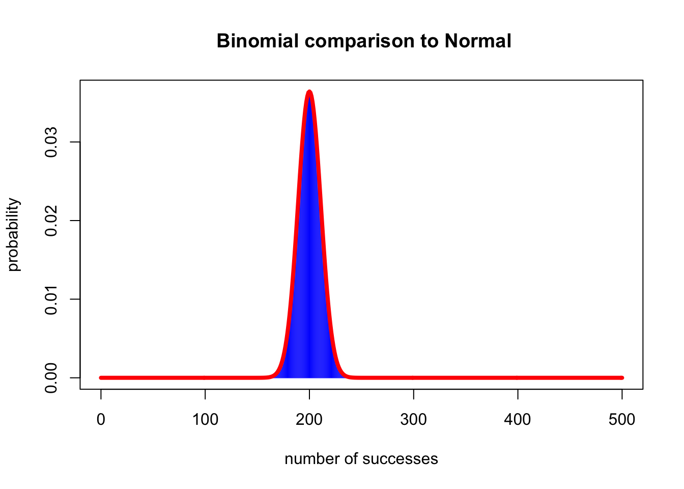
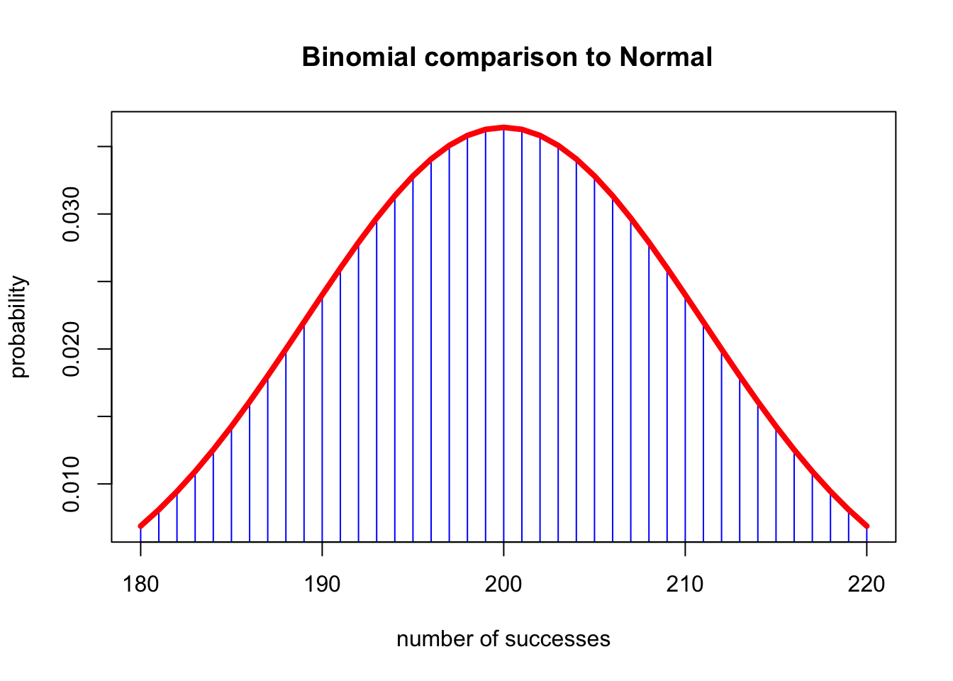
- When \(n\), \(n \pi\), and \(n(1-\pi)\) are sufficiently large, then the binomial distribution is well approximated by the normal distribution.
plot(0:500, dbinom(0:500, 500, 0.4),
     type = "h",
     col = "blue",
     xlab = "number of successes",
     ylab = "probability",
     main = " Binomial comparison to Normal")
lines(0:500, dnorm(0:500, 200, sqrt(500 * 0.4 * 0.6)), lwd = 4, col = "red")
plot(180:220, dbinom(180:220, 500, 0.4), type = "h", col = "blue", xlab = "number of successes",
    ylab = "probability", main = " Binomial comparison to Normal")
lines(180:220, dnorm(180:220, 200, sqrt(500 * 0.4 * 0.6)), lwd = 4, col = "red")
- The closer \(\pi\) is to 0.5, the
better the normal approximation will be.
- If \(n \le 50\), the approximation will not be good
- Rule of thumb: \(n \pi(1-\pi) \ge 10\)
5.1 Implications for the confidence interval for the sampling propotion
- If \(n \pi(1-\pi) \ge 10\) (i.e., sufficiently large), the sampling distribution for the sample proportion can be approximated by a normal distribution with mean \(\pi\) and standard deviation of \(\sqrt{(\pi(1-\pi) / n)}\).
- So for large \(n\) (i.e., \(n \pi(1-\pi) \ge 10\)), an approximate 100(1-\(\alpha\))% confidence interval for \(\pi\), can be determined with a normal distribution.
5.2 Example: Approximation of 95% Confidence Interval for the population proportion
\[ 0.95=\operatorname{Pr}\left(q_{0.025} \leq \frac{p-\pi}{\sqrt{p(1-p) / n}} \leq q_{0.975}\right) \]
- The quantity given above has a standard normal distribution.
R
qnorm(0.025)## [1] -1.959964qnorm(0.975)## [1] 1.959964\[ 0.95=\operatorname{Pr}\left(p-q_{0.975} \sqrt{p(1-p) / n} \leq \pi \leq p+q_{0.975} \sqrt{p(1-p) / n}\right) \]
\[ 0.95=\operatorname{Pr}(p-1.96 \sqrt{p(1-p) / n} \leq \pi \leq p+1.96 \sqrt{p(1-p) / n}) \]
- e.g. Suppose we have a random sample of 500 individuals from a population and that 212 of them are obese (e.g. have a BMI > 30).
- <1> What is an estimate for the proportion of obese individuals in this population?
binom.test(212, 500, conf.level = 0.90)##
## Exact binomial test
##
## data: 212 and 500
## number of successes = 212, number of trials = 500, p-value = 0.0007798
## alternative hypothesis: true probability of success is not equal to 0.5
## 90 percent confidence interval:
## 0.3870533 0.4616173
## sample estimates:
## probability of success
## 0.424- <2> What is the 90% confidence interval obtained from a normal approximation?
(lower <- 0.424 - 1.645 * sqrt(0.424 * 0.576 / 500)) %>% round(3)## [1] 0.388(upper <- 0.424 + 1.645 * sqrt(0.424 * 0.576 / 500)) %>% round(3)## [1] 0.46(test <- prop.test(212, 500, conf.level = 0.90))##
## 1-sample proportions test with continuity correction
##
## data: 212 out of 500, null probability 0.5
## X-squared = 11.25, df = 1, p-value = 0.0007962
## alternative hypothesis: true p is not equal to 0.5
## 90 percent confidence interval:
## 0.3871687 0.4616718
## sample estimates:
## p
## 0.424- Using the
prop.test()the 90% CI is 0.387, 0.462.
Rfunction gives more accurate estimates is that it uses a correction for continuity. Specifically the binomial distribution is discrete and the normal distribution is continuous so a correction is needed to assign the area under the curve (AUC) to each mass of the binomial.