1. Type I and Type II Error
1.1 Hypothesis test review
- \(H_0\): \(\theta\)=\(\theta_0\)
- \(H_a\): \(\theta \ne \theta_0\).
- Given a test statistic, the null distribution of the statistic, and a significant level, we are able to determine if we have enough evidence in the data to reject the null hypothesis.
1.2 Errors
- When testing hypothesis, there are two possible errors that we can
make:
- Type I error: Rejecting the null when the null hypothesis is true.
- Type II error: Not rejecting the null when the null hypothesis is false.
| Test vs. truth | \(H_0\) is true | \(H_0\) is false |
|---|---|---|
| Reject \(H_0\) | Type I error | Correct |
| Do not reject \(H_0\) | Correct | Type II error |
- In classical statistics, we want to minimize the type I error, by setting a threshold to limit it to a pre-specified acceptable value, say 5%.
- The significance level of a test is the \(\alpha\) that we find acceptable for the probability of a type I error.
- Good scientific and statistical practice is to set this value at the time you are designing the study, well before you look at any study data.
- The definition of type I error (or the level of significance) is
\[ \alpha=\operatorname{Pr}\left(\text { Reject } H_{0} \mid H_{0} \text { is true }\right) \]
We can control the probability of a type I error by setting the significance level, \(\alpha\).
The definition of type II error is:
\[ \beta=\operatorname{Pr}\left(\text { Do not reject } H_{0} \mid H_{0} \text { is false }\right) \]
- If we are just given a set of data, we can control the type I errors by setting the \(\alpha\) as we are planning the analysis, before we look at the data.
- However in this case, we do not have control over the probability of
a type II error and we just accept its value.
- However, if we are designing a study from scratch, we can set both the type I error and type II error and determine the sample size needed to achieve these values.
Study design 단계에서부터 필요한 sample size를 구하고 들어오면, type I and type II error 모두 control 가능함
1.3 Power
- Usually, we are not interested directly in the type II error, but in its complement,
\[ 1-\beta=\operatorname{Pr}\left(\text { Reject } H_{0} \mid H_{0} \text { is false }\right)=\text { power } \]
- This is called the power of the test: the probability of correctly rejecting the null hypothesis when it is false.
| Test vs. Truth | \(H_0\) is true | \(H_0\) is false |
|---|---|---|
| Reject \(H_0\) | \(\alpha\) (Type I error) | \(1-\beta\) (Power) |
| Do not reject \(H_0\) | \(1-\alpha\) | \(\beta\) (Type II error) |
1.4 Illustration of type I and type II error
- Can use density plots to illustrate the relationship of \(\alpha\), power \((1-\beta)\) and the null and alternative hypotheses.
curve(dnorm, from = -3, to = 3,
      xlim = c(-3, 6),
      lwd = 2, col = 4,
      axes = F, xlab = NA, ylab = NA)
curve(dnorm(x, mean = 3.2),
      add = TRUE, col = 2, lwd = 2, from = 0, to = 6)
coord.x <- c(qnorm(0.95), seq(qnorm(0.95), 6, by = 0.01), 6)
coord.y <- c(0, dnorm(coord.x[-c(1, length(coord.x))], mean = 3.2), 0)
polygon(coord.x, coord.y, col = rgb(1, 0, 0, 0.5))
coord.x <- c(qnorm(0.95), seq(qnorm(0.95), 3, by = 0.01), 3)
coord.y <- c(0, dnorm(coord.x[-c(1, length(coord.x))]), 0)
polygon(coord.x, coord.y, col = rgb(0, 0, 1, 0.5))
abline(v = qnorm(0.95), lty = 2, lwd = 2)
text(3.2, 0.2, labels = expression(1 - beta))
text(2, 0.02, labels = expression(alpha), col = "white")
axis(1, at = c(0, 3.2), labels = c(expression(theta[0]), expression(theta[1])))
axis(2)
box()
legend("topleft",
       c("Distribution under H0",
         "Distribution under H1",
         "Critical value"),
       bg = "transparent",
       lty = c(1, 1, 2),
       col = c(4, 2, 1), lwd = 2)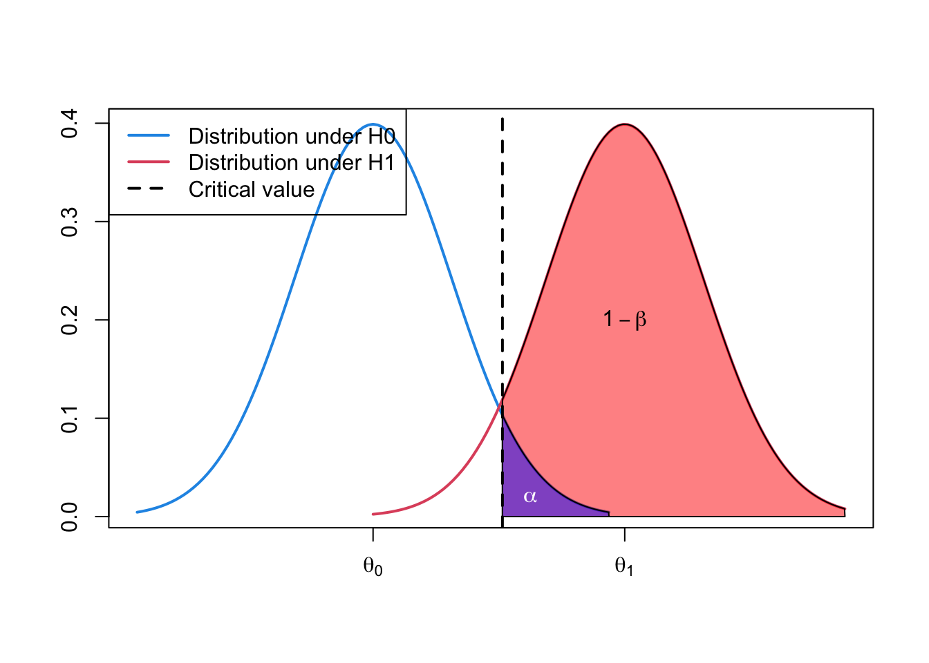
curve(dnorm, from = -3, to = 3,
      xlim = c(-3, 6),
      lwd = 2, col = 4, axes = FALSE,
      xlab = NA, ylab = NA)
curve(dnorm(x, mean = 3.2),
      add = TRUE, col = 2, lwd = 2,
      from = 0, to = 6)
coord.x <- c(qnorm(0.95), seq(qnorm(0.95), 0, by = -0.01), 0)
coord.y <- c(0, dnorm(coord.x[-c(1, length(coord.x))], mean = 3.2), 0)
polygon(coord.x, coord.y, col = rgb(1, 0, 0, 0.5))
coord.x <- c(qnorm(0.95), seq(qnorm(0.95), 3, by = 0.01), 3)
coord.y <- c(0, dnorm(coord.x[-c(1, length(coord.x))]), 0)
polygon(coord.x, coord.y, col = rgb(0, 0, 1, 0.5))
abline(v = qnorm(0.95), lty = 2, lwd = 2)
text(1, 0.02, labels = expression(beta))
text(2, 0.02, labels = expression(alpha), col = "white")
axis(1, at = c(0, 3.2),
     labels = c(expression(theta_0), expression(theta_a)))
axis(2)
box()
legend("topleft",
       c("Type I error", "Type II error"),
       fill = c(rgb(0, 0, 1, 0.5),
                rgb(1, 0, 0, 0.5)))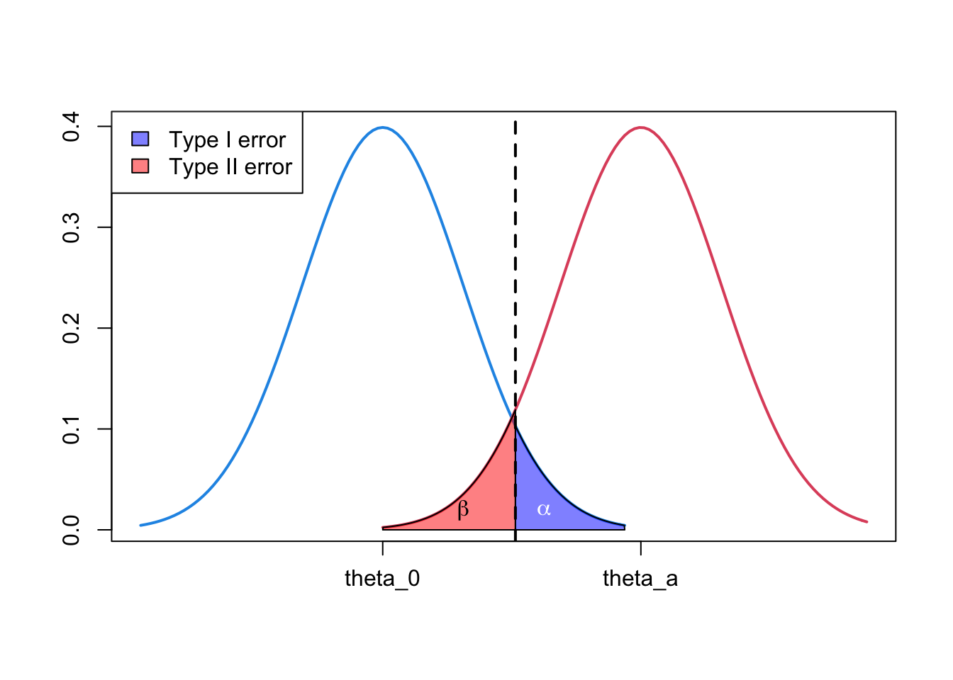
curve(dnorm, from=-3, to=3,
      xlim=c(-3, 6), lwd=2, col=4,
      axes=FALSE, xlab=NA, ylab=NA)
curve(dnorm(x, mean=3.2),
      add=TRUE, col=2, lwd=2,
      from=0, to=6)
coord.x <- c(qnorm(0.9), seq(qnorm(0.9), 0, by=-0.01), 0)
coord.y <- c(0, dnorm(coord.x[-c(1, length(coord.x))], mean=3.2), 0)
polygon(coord.x, coord.y, col=rgb(1, 0, 0, 0.5))
coord.x <- c(qnorm(0.9), seq(qnorm(0.9), 3, by=0.01), 3)
coord.y <- c(0, dnorm(coord.x[-c(1, length(coord.x))]), 0)
polygon(coord.x, coord.y, col=rgb(0, 0, 1, 0.5))
abline(v = qnorm(0.9), lty=2, lwd=2)
text(1, 0.02, labels = expression(beta))
text(2, 0.02, labels = expression(alpha), col = "white")
axis(1, at = c(0, 3.2), labels = c(expression(theta_0), expression(theta_a)))
axis(2)
box()
legend("topleft",
       c("Type I error", "Type II error"),
       fill = c(rgb(0, 0, 1, 0.5),
                rgb(1, 0, 0, 0.5)))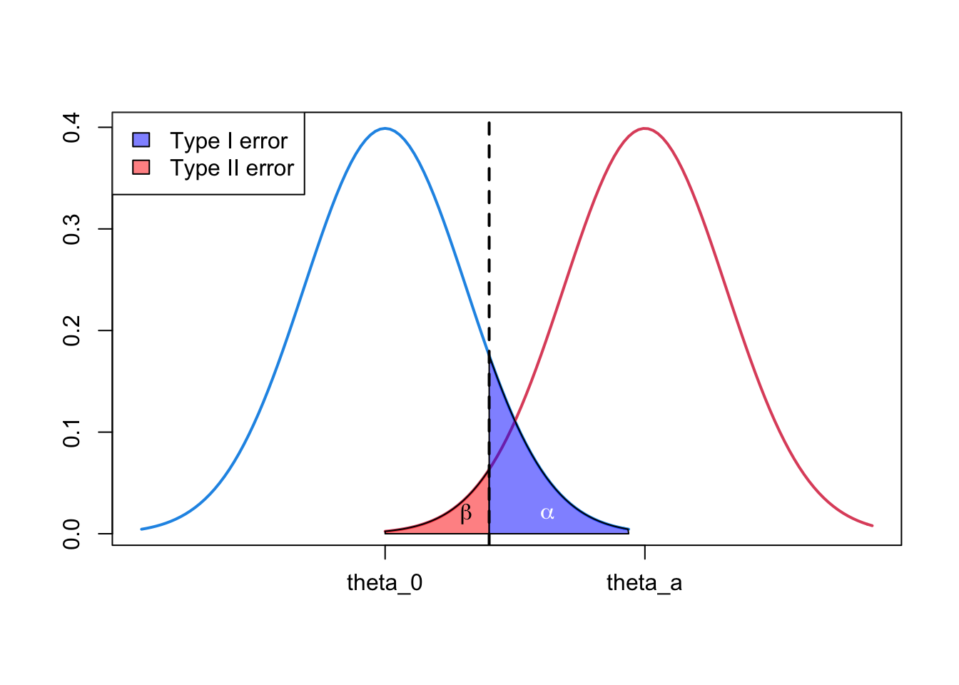
curve(dnorm,
      from=-3, to=3,
      xlim=c(-3, 6), lwd=2, col=4,
      axes=FALSE, xlab=NA, ylab=NA)
curve(dnorm(x, mean=3.2),
      add=TRUE, col=2, lwd=2,
      from=0, to=6)
coord.x <- c(qnorm(0.99), seq(qnorm(0.99), 0, by=-0.01), 0)
coord.y <- c(0, dnorm(coord.x[-c(1, length(coord.x))], mean=3.2), 0)
polygon(coord.x, coord.y, col=rgb(1, 0, 0, 0.5))
coord.x <- c(qnorm(0.99), seq(qnorm(0.99), 3, by=0.01), 3)
coord.y <- c(0, dnorm(coord.x[-c(1, length(coord.x))]), 0)
polygon(coord.x, coord.y, col=rgb(0, 0, 1, 0.5))
abline(v = qnorm(0.99), lty=2, lwd=2)
text(1.6, 0.02, labels = expression(beta))
text(2.5, 0.015, labels = expression(alpha), col = "white")
axis(1, at = c(0, 3.2), labels = c(expression(theta_0), expression(theta_a)))
axis(2)
box()
legend("topleft",
       c("Type I error", "Type II error"),
       fill = c(rgb(0, 0, 1, 0.5),
                rgb(1, 0, 0, 0.5)))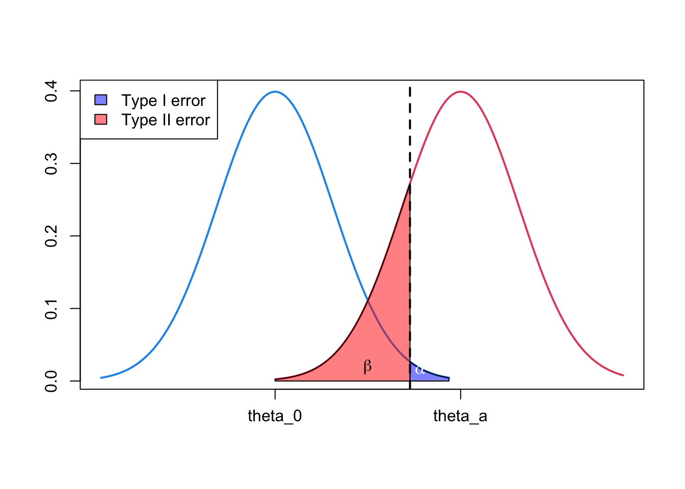
2. Example: Binomial distribution
- simple random sample from a population with two outcomes (success and failure), with unknown probability of success \(\pi\)
y <- rbinom(100, 1, 0.5)- to test
- \(H_0: \pi= \pi_0=0.5\)
- \(H_a: \pi= \pi_a>0.5\) (one-sided)
- Under \(H_0\), \(P\) has a rescaled \(B(100, \pi_0)\) distribution.
- Under \(H_a\), \(P\) has a rescaled \(B(100, \pi_a)\) distribution.
- (One-sided test) Rejection region: \((c,
+\infty)\)
- where \(c\) is called the critical value
- Since the sampling distribution of \(P\) is a rescaled binomial, we can express \(c\) either on the proportion scale or on the number of successes scale.
- Suppose we fix \(\alpha\), then the critical value can be computed from the binomial distribution:
\[ \operatorname{Pr}\left(Y>y_{1-\alpha} \mid H_{0}\right)=\alpha \]
- When \(Y~B(n, \pi_0)\), then \(P=Y/n\)
- The rejection region is 95th percentile of the binomial distribution.
(q <- qbinom(0.95, 100, 0.5))## [1] 58- Therefore, the **rejection region on the number of successes scale is \(Y>58\) or on the sample proportion scale (\(P\) scale) is:
\[ \begin{array}{c}Y>58 \\ Y / 100>58 / 100 \\ P>0.58\end{array} \]
- The plot of the null distribution and the critical value on the sample proportion scale
pi_0 <- 0.5
n <- 100
plot((20:80)/100,dbinom(20:80, n, pi_0),
     type = "h",lwd=2,
     main="Rejection region",
     xlab = "sample proportion",
     ylab="PMF")
abline(v = 0.58, lty=2, lwd=2, col=3)
lines((58:80)/100, dbinom(58:80,n, pi_0),
      type = "h", lwd=4, col=4)
legend("topright",
       c("Null distribution", "Critical value"),
       lwd=2, lty=c(1, 2), col=c(1, 3))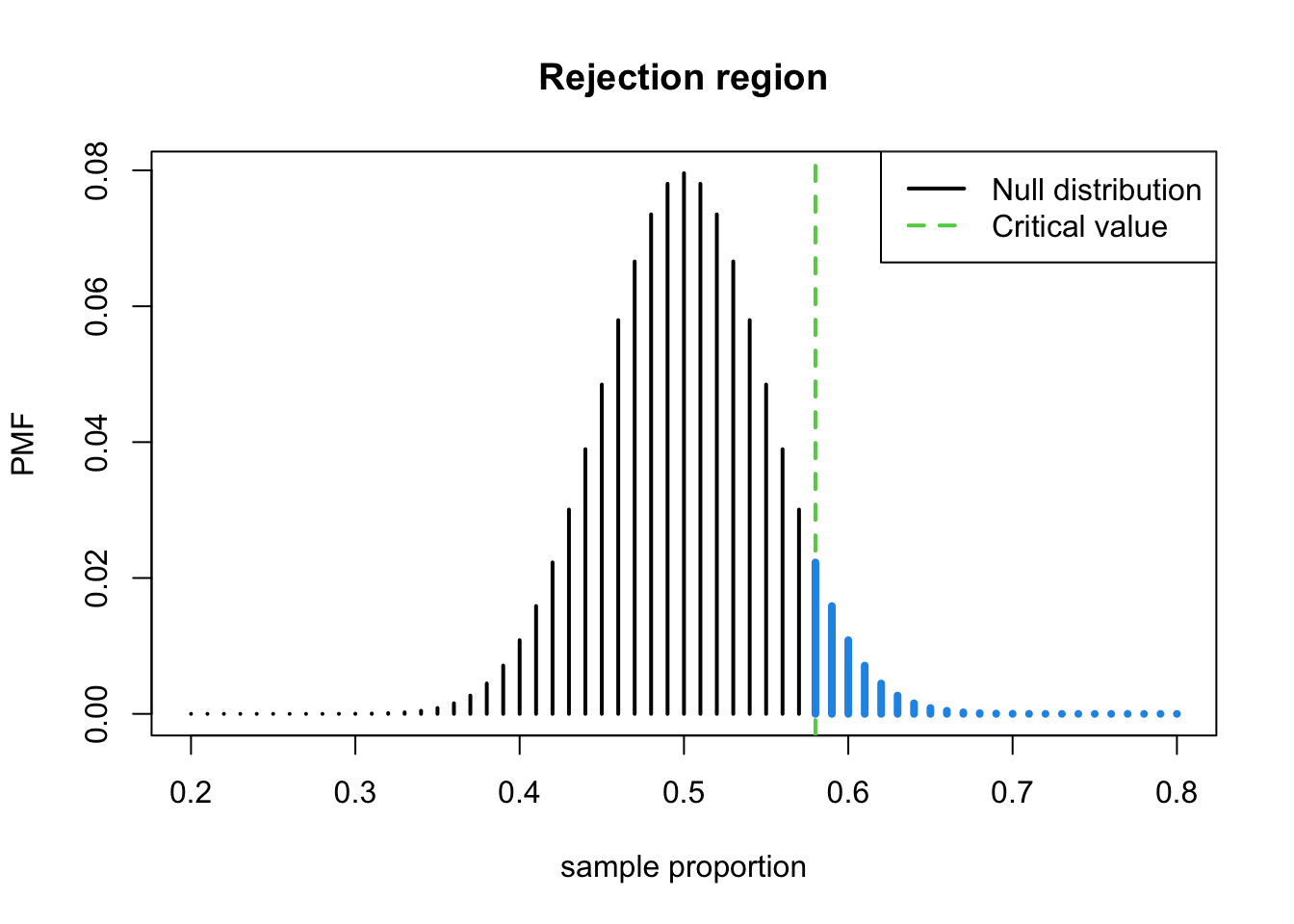
- The probability of the blue region is approximately 0.05.
2.1 Power
- Power = \(1-\beta\)
- In order to compute the power, we have to assume a specific value
for the alternative distribution.
- In this case, presume that the researchers believe that \(\pi_a=0.6\).
- This corresponds to a sample proportion of 0.60 or a \(Y\) value of \(Y=100 \times \pi_a=60\).
\[ 1-\beta=\operatorname{Pr}\left(\text { Reject } H_{0}|H_{a})=\operatorname{Pr}\left(Y>58 \mid \pi_{a}=0.6\right)\right. \]
R:pbinom()
(1 - pbinom(58, 100, 0.6)) %>% round(3)## [1] 0.623Therefore, the chance we will get a statistically significant result (meaning a \(p\)-value < \(\alpha=0.05\)) **if the alternative hypothesis is true (i.e. under the alternative hypothesis) (e.g. \(\pi_a=0.60\)) is 0.623.
The plot of power, the sum of the red bars for the \(H_a\) PMF is the power
pi.0 <- 0.5
pi.a <- 0.6
n <- 100
plot((20:80)/100,dbinom(20:80, n, pi.0),
     type = "h",lwd=5, main="Power",
     xlab = "sample proportion", ylab="PMF")
lines((20:80)/100,
      dbinom(20:80,n, pi.a),
      type = "h", lwd=2, col="orange")
lines((59:80)/100,
      dbinom(59:80,n, pi.a),
      type = "h", lwd=2, col="orangered3")
abline(v = 0.58, lty=2, lwd=4, col=3)
legend("topleft",
       c("Null distribution",
         "Alternative distribution",
         "Critical value"),
       lwd=2, lty=c(1, 1, 2),
       col=c(1, "orange", 3))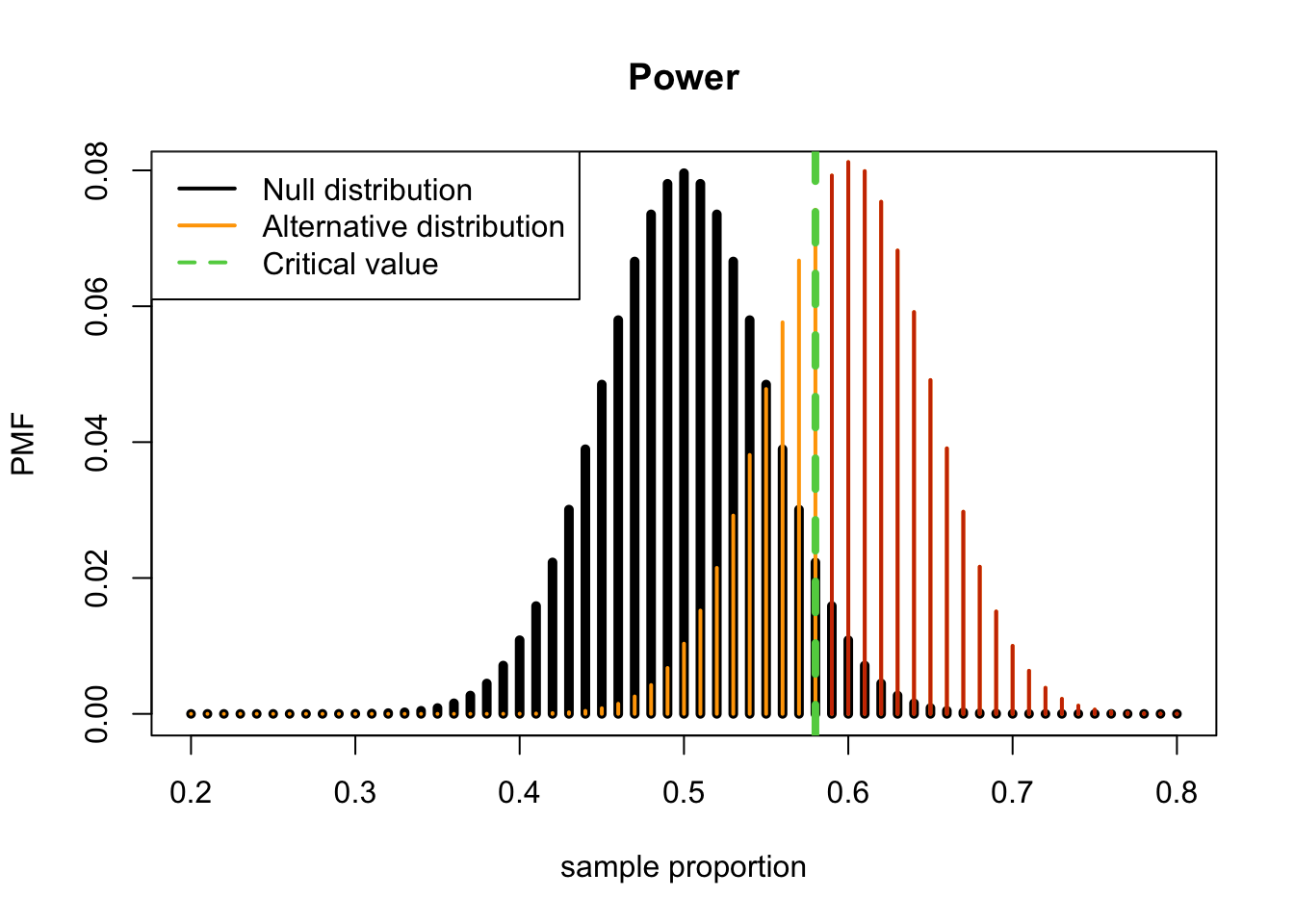
Conclusion: We have 62.3% power to reject \(H_0: \pi=0.5\) when the true population proportion is \(\pi=0.60\) with a sample size of \(n\) and a 5% (one-sided) level of significance.
Rfunction to calculate the power:propTestPower()in theEnvStatspackage.
library(EnvStats)## Warning: package 'EnvStats' was built under R version 4.0.5##
## Attaching package: 'EnvStats'## The following object is masked from 'package:MASS':
##
## boxcox## The following objects are masked from 'package:moments':
##
## kurtosis, skewness## The following objects are masked from 'package:stats':
##
## predict, predict.lm## The following object is masked from 'package:base':
##
## print.default- To get the power using an exact binomial
distribution: set the argument to
approx = FinpropTestPower().approx = Twill make the function use a normal approximation to the binomial to determine the power.
samplePower <- propTestPower(100,0.6, 0.5,
                             alpha=0.05,
                             sample.type = "one.sample",
                             alternative = "greater",
                             approx=FALSE)
samplePower
## $power
## [1] 0.6225327
##
## $alpha
## [1] 0.04431304
##
## $q.critical.upper
## [1] 58- Due to the discreteness of the binomial distribution, the \(\alpha\) is not exactly equal to the specified value.
- Conclusion: Using one-sided level of significance of 0.05 with a sample size of \(n\), there is 62.3% probability to detect a \(\pi_a=0.60\). The critical value is 58, meaning that if we observe more than this many successes, 58, we would reject the null hypothesis, \(H_0\).
- We DO NOT use the values of the sample in any of our calculations.
- This means we can compute the power of a test BEFORE performing the experiment.
- The power is actually determined during study design.
- It is not particularly useful to determine power after you have your data.
- The power associated with a sample can be better conveyed by presenting the confidence interval for your estimate.
- If the confidence interval is wide, this means that the study did not have very high power.
3. Power
3.1 Power curve
- So far, we have been interested in testing hypotheses, \(H_a: \pi>\pi_0\), where there are many
values of \(\pi\) under \(H_a\).
- Also, \(H_a:\pi<\pi_0\).
R: the power of a range of values of \(\pi_a\)
pi.a <- seq(0, 1, by = 0.01)
power <- 1 - pbinom(qbinom(0.95,100,0.5), 100, pi.a)

# Power curve with the sample size of n=100 for a population proportion
plot(pi.a, power,
     type='s', lwd=2,
     ylab=expression(1-beta),
     xlab=expression(pi))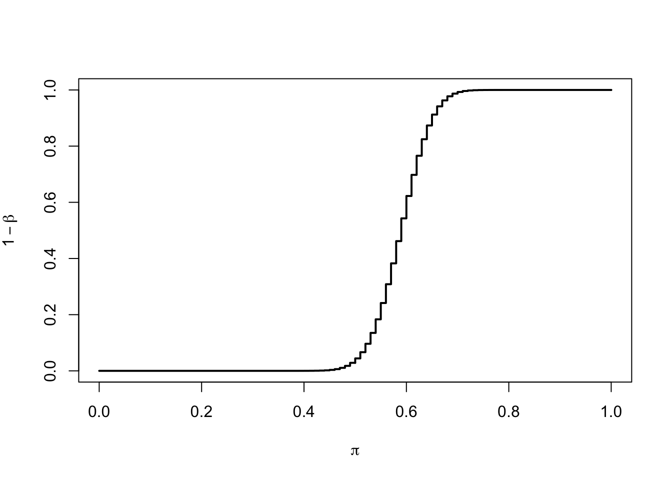
- Features of the power curve:
- <1> the curve converges to \(\alpha=0.05\) when \(\pi\) gets closer to \(\pi_0=0.5\)
- <2> the power increases with the distance between \(\pi\) and \(\pi_0\)
- <3> the curve converges to 1 as \(\pi\) gets further from \(\pi_0\)
3.2 Power and sample size
- Power depends on the sample size.
- By increasing the number of observations in the sample, we can increase the power of the test (i.e., \(1-\beta\) or decreasing the Type II error).
- The power of the test is important in order to understand what magnitude of effects we will be able to test.
- In particular, this is important for studies that do not have a
statistically significant result.
- Because the studies that have a statistically significant reuslt already have enough power.
- (\(p\)-value > \(\alpha\)) the result is said not to be statistically significant.
- The question is
- whether this is because \(H_0\) is true, or
- because we did not have enough power to detect a difference of interest.
- Often, researchers decide what power they need to test a given effect size and plan to collect a sample of a size \(n\) that will give them enough power.
R: the plot of the power of a test as a function of sample size
pi.a50 <- seq(0, 1, by = 0.02)
pi.a100 <- seq(0, 1, by = 0.01)
pi.a200 <- seq(0, 1, by = 1/200)

power50 <- 1 - pbinom(qbinom(0.95,50,0.5), 50, pi.a50)
plot(pi.a50, power50, type='s', ylab=expression(1-beta), xlab=expression(pi), lwd=2)

power100 <- 1 - pbinom(qbinom(0.95,100,0.5), 100, pi.a100)
lines(pi.a100, power100, type='s', col=3, lwd=2)

power200 <- 1 - pbinom(qbinom(0.95,200,0.5), 200, pi.a200)
lines(pi.a200, power200, type='s', col=6, lwd=2)

legend("bottomright", paste0("n = ", c(50,100,200)), lwd=2, col=c(1,3,6))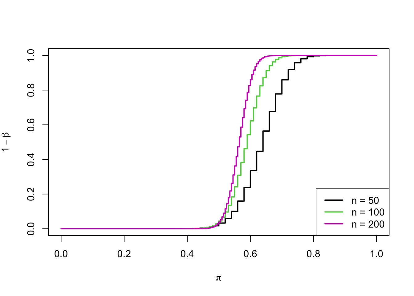
3.3 What do we know?
- In general we know \(\pi_0\) and \(\alpha\).
- \(\pi_0\) is often based on historical data and the research team determines the \(\alpha\) they want to use.
- In order to compute this power, we need to specify
two of the following three:
- \(n\), \(\beta\), \(\pi_a\)
- Usually, we want to know what is the power for a given \(\pi_a\) and \(n\) or
- we want to know what sample size \(n\) we need to obtain a certain power, \(1-\beta\), and \(\pi_a\).
3.4 Effect size
- Power depends only on:
- \(n\), the sample size
- the difference between the null and alternative proportions also known as effect size
3.5 Power and sample size (given \(\pi_a\) and \(n\))
- What is the samllest sample size \(n\) that we need to achieve a given power?
- Very common question in biostatistics
- Because when we are testing experimental treatments on patients, we do not want to harm patients unnecessarily.
It is a moral obligation to:
- <1> collect a sample size large enough to be able to prove an effect if there is one.
- <2> collect a sample size small enough to avoid potentially harming many people.
- This process is generally refeered to as power calculation
- It involves making decisions on:
- \(\alpha\): a significance level
- \(\pi_a\): we want to be able to detect
- \(1-\beta\): the power of the test
- Example: suppose that we want a 80% chance to reject \(H_0: 0.5\) at \(\alpha=0.01\) if the true proportion is \(\pi_a=0.65\) with one-sided test. What is the smallest sample size \(n\) that we need?
- The given information is:
- \(1-\beta=0.80\)
- \(\pi_a=0.5\)
- \(\alpha=0.01\)
- \(\pi_a=0.65\)
R:propTestN
sampleSize <- propTestN(0.65, 0.5, alpha = 0.01, power = 0.80,
                        sample.type = "one.sample",
                        alternative = "greater",
                        approx=FALSE)
sampleSize
## $n
## [1] 114
##
## $power
## [1] 0.817283
##
## $alpha
## [1] 0.009405374
##
## $q.critical.upper
## [1] 69- Set
approx=F: the function compute the sample size using the exact binomial.approx=T: the function uses a normal approximation to the binomial.
- Since the function uses an exact binomial, it is not possible
sometimes to get the exact power and \(\alpha\) that are stated.
- This is because of the discreteness of binomial distribution.
- The program determines the value as close as possible doing a search.
- Conclusion: the required sample size would be 114 with one-sided \(alpha=0.01\) and power of 81.7%.
3.6 What is the minimum detectable difference? (given \(n\), power)
propTestMddin theEnvStatspackage is the function to determine the minimum detectable difference if the sample size \(n\) is known and for a desired level of power.- e.g. Suppose we have a sample size 100 and want 90% power with \(alpha=0.05\), one-sided significance.
propDetectDiff <- propTestMdd(100, 0.50, alpha = 0.05, power = .9,
                              sample.type = "one.sample",
                              alternative = "greater",
                              approx=FALSE)
propDetectDiff
## $delta
## [1] 0.1465346
##
## $power
## [1] 0.9
##
## $alpha
## [1] 0.04431304
##
## $q.critical.upper
## [1] 58- Since the function is using an exact binomial, it is not possible
sometimes to get the exact \(alpha\)
that was stated.
- This is because of the discreteness of a binomial distribution.
- The program determines the value as close as possible doing a search.
- Conclusion: for a power of 90% and a sample size of 100, the minimum detectable difference is 0.15 with one-sided \(\alpha=0.01\).
3.7 Summing up
- As the difference between means increases, power increases.
- As the sample size increases, power increases.
- As the significance level increases, power increases.
- To compute the sample size, for a single population
proportion using an exact binomial, use
propTestN().- You need power, significance level \(\alpha\), and the difference to detect.
- To compute the power for a sample of a single
population proportion using an exact binomial, use
propTestPower().- You need the sample size \(n\), significance level \(\alpha\), and the difference to detect.
- To compute the minimal detectable difference for a
single population proportion using an exact binomal, use
propTestMdd().- You need the sample size \(n\), significance level \(\alpha\), and the power.