1. Pharmacology example
One method for assessing the bio availability of a drug is to note
its concentration in blood and/or urine samples at certain period of
time after the drug is given. Suppose we want to compare the
concentrations of two types of aspirin (Types A and B) in urine
specimens taken from the the same person 1 hour after she or he has
taken the drug. Hence, a specific dosage of either Type A or Type B
aspirin is given at one time and the 1-hour urine concentration is
measured. One week later, after the aspirin has presumably been cleared
from the system, the same dosage of the other aspirin is given to the
same person and the 1-hour urine concentration is noted. Because the
order of giving the drugs may affect the result, patients were
randomized to either take A first (then one week later B) or to take B
first (and then one week later A). This experiment was performed on 25
people. The data are found in a file called aspirin.csv.
Read the data into R and save in an object called
aspirinPharm.
aspirinPharm <- read.csv("./data/aspirin.csv")
head(aspirinPharm)
## subjID Avals Bvals
## 1 s372 22.0 20.0
## 2 s268 24.9 16.1
## 3 s281 23.1 29.1
## 4 s328 10.0 12.8
## 5 s314 18.8 16.9
## 6 s384 36.1 18.0The column Avals contains the aspirin A 1-hour
concentration (mg%) and the column Bvals contains the
aspirin B 1-hour concentration (mg%). The column subjID is
the id number of the subject.
2. Approximate sampling distribution
- We are interested in the mean concentration levels of each of the different aspirins.
- Our focus will first be on Aspirin A. We are interested in \(\mu\), the true mean concentration level for aspirin A.
- Intuitively, we would use the sample mean to estimate \(\mu\).
- Specifically the sample mean would be obtained with the
Rfunctionmean(). - In this case, the sample mean is 20.9.
- However, we know that the sample mean likely will not equal the population mean, \(\mu\).
- Specifically, different samples of the same sample sizes will yield different sample means.
- The question is **how can we gauge the accuracy of 20.9 as an estimate of \(\mu\)?
2.0 Sampling distribution
- If we had the sampling distribution for the sample means for samples of size 25 from the population, then this would give us an idea of how the sample means vary from sample to sample.
- Looking at the spread of the sampling distribution of the sample means, measured by the standard deviation, we can get a sense of how far sample means can deviate from the population mean, \(\mu\).
- However, since we cannot afford to give aspirin A to the entire population and measure the concentrations, we cannot generate the sampling distribution.
Note if we did give aspirin A to the entire population and measured the concentrations in the urine, we would know the population mean value!
2.1 Review bootstrap distribution
- Bootstrap is a procedure that uses the given sample to create a bootstrap distribution, that approximates the sampling distribution for the sample statistic, which in this case would be the sample mean.
- We’ll use a small subset of the urine concentrations levels: 22, 24.9, 23.1.
- To find the bootstrap distribution of the mean,
- draw samples (bootstrap sample) of size \(n\), with replacement, from the original sample and then
- compute the mean of each resample.
- The original sample of size 3 is the population.
- There are \(3^3=27\) samples of size 3, taking order in which they are drawn into account.
- From this, we can compute the sample mean for each of the 27 samples.
- All 27 samples of size 3
- \(x_1^*\): resampled observation
- \(x_2^*\): resampled observation
- \(x_3^*\): resampled observation
- \(\bar{x^*}\): statistic of interest (sample mean in this case)
\[ \begin{array}{llll}\hline x_{1}^{*} & x_{2}^{*} & x_{3}^{*} & \bar{x}^{*} \\ \hline 22.0 & 22.0 & 22.0 & 22.0 \\ 22.0 & 22.0 & 24.9 & 23.0 \\ 22.0 & 22.0 & 23.1 & 22.4 \\ 22.0 & 24.9 & 22.0 & 23.0 \\ 22.0 & 24.9 & 24.9 & 23.9 \\ 22.0 & 24.9 & 23.1 & 23.3 \\ 22.0 & 23.1 & 22.0 & 22.4 \\ 22.0 & 23.1 & 24.9 & 23.3 \\ 22.0 & 23.1 & 23.1 & 22.7 \\ 24.9 & 22.0 & 22.0 & 23.0 \\ 24.9 & 22.0 & 24.9 & 23.9 \\ 24.9 & 22.0 & 23.1 & 23.3 \\ 24.9 & 24.9 & 22.0 & 23.9 \\ 24.9 & 24.9 & 24.9 & 24.9 \\ 24.9 & 24.9 & 23.1 & 24.3 \\ 24.9 & 23.1 & 22.0 & 23.3 \\ 24.9 & 23.1 & 23.1 & 23.7 \\ 24.9 & 23.1 & 24.9 & 24.3 \\ 23.1 & 22.0 & 22.0 & 22.4 \\ 23.1 & 22.0 & 24.9 & 23.3 \\ 23.1 & 22.0 & 23.1 & 22.7 \\ 23.1 & 24.9 & 22.0 & 23.3 \\ 23.1 & 24.9 & 24.9 & 24.3 \\ 23.1 & 24.9 & 23.1 & 23.7 \\ 23.1 & 23.1 & 22.0 & 22.7 \\ 23.1 & 23.1 & 24.9 & 23.7 \\ 23.1 & 23.1 & 23.1 & 23.1 \\ \hline\end{array} \]
R: the sampling distribution is based on a sample of size 3.
sample <- aspirinPharm$Avals[1:3] # c(22, 24.9, 23.1)

hist(xbarDist, freq=F, xlab="sample mean", ylab="proportion", main="Sample Distribution for Sample Mean (n = 3)", col="lavender", breaks = 6)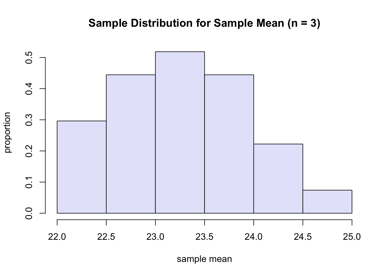
- The idea behind the bootstrap is that
- if the original sample is representative of the population, then the bootstrap distribution of the mean will look approximately like the sampling distribution of the mean;
- that is, have roughly the same spread and shape.
- However, the mean of the bootstrap distribution will be the same as
the mean of the original sample, but not necessarily that of the
original population.
- Thus, in the lecture 7, we already said that the bootstrap distribution is not a good estimate of population mean.
- Summary:
- can use the bootstrap sample to approximate the spread of the real sampling distribution and to approximate the shape of the real sampling distribution.
- cannot use it to approximate the population mean, \(\mu\).
- To estimate the population mean, \(\mu\), we will use the sample mean of the original sample. (point estimate)
Bootstrap Idea
- The original sample approximates the population from which it is drawn.
- Resamples from this sample approximate what we would get if we took many samples from the population.
- The bootstrap distribution of a statistic, based on many resamples, approximates the sampling distribution of the statistic, based on many samples.
- Now let’s work with the full data set.
- Draw resamples of size \(n=25\) from the 25 concentration levels for aspirin A and calculate the mean for each.
- There are now \(25^25\) samples. (too many)
- Instead we draw samples randomly, of size 25, with replacement, from the data, and calculate the mean for each.
- We repeat this process many times, say \(B=7500\), to create the bootstrap distribution.
- Imagine that there is a table similar to the one above but with \(25^25\) rows (as a sample space).
- We will randomly pick 7500 rows out of \(25^25\) rows.
Bootstrap for a Single Population
- Given a sample of size \(n\) from a population.
- <1> Draw a resample of size \(n\) with replacement from the sample. Compute a statistic that describes the sample such as the sample mean.
- <2> Repeat the resampling process many times, say between 5000 and 10000.
- <3> Construct the bootstrap distribution of the statistic. Inspect its spread, bias, and shape.
2.2 Example
For our example, we would estimate the mean urine concentration 1-hour after ingesting aspirin A using the sample mean, 20.9. In addition to the point estimate, we would like a 90% confidence interval. Since we do not know the sample distribution for the sample mean, we will do a bootstrap. Specifically, we will estimate the sampling distribution for the sample mean based on \(B=7500\) bootstrapped samples.
- ‘manual’ bootstrapped sample and its distribution
B <- 7500
n <- length(aspirinPharm$Avals)
xbar <- replicate(B,
                  {
                    x <- sample(aspirinPharm$Avals, size = n, replace = T)
                    mean(x)
                    }
                  )
hist(xbar, probability = T, breaks=20,
col="lemonchiffon",
xlab="sample mean",
ylab = "probability",
main = "Estimate of the sampling distribution of sample mean")
lines(density(xbar), col=2, lwd=3)
legend("topright", "density", col=2, lwd=3)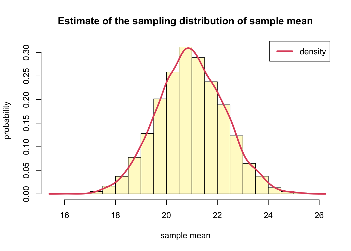
- the sample mean of the approximate sampling distribution of the sample mean and the standard deviation of the sampling distribution of the sample mean (i.e. standard error)
# mean
mean(xbar) %>% round(1)
## [1] 21# standard deviation
sd(xbar) %>% round(2)## [1] 1.31- compare the distribution of the original sample to that of the approximation of the sample distribution for the sample mean.
par(mfrow = c(1,2))
hist(aspirinPharm$Avals, freq = F, breaks = 10,
     xlim=c(min(aspirinPharm$Avals),
            max(aspirinPharm$Avals)),
     col="lemonchiffon",
     xlab="concentration",
     ylab = "probability",
     main = "Concentrations Disribution")
lines(density(aspirinPharm$Avals), col=6, lwd=3)
hist(xbar, probability = T, breaks=20,
     xlim=c(min(aspirinPharm$Avals),
            max(aspirinPharm$Avals)),
     col="lemonchiffon",
     xlab="sample mean",
     ylab = "probability",
     main = "Sample Dist of Sample Mean")
lines(density(xbar), col=6, lwd=3)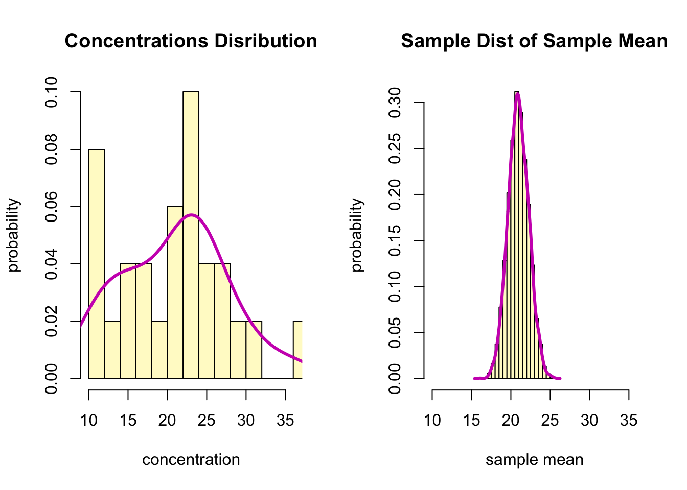
- According to the two histograms, the bootstrap distribution of the sample mean is approximately normal.
- With mean 20.9, it is centered at approximately at the same location as the original mean, 20.9
- We get a rough idea of the amount of variability.
- We can quantify the variability by computing the **standard deviation of the bootstrap distribution, 1.31 in this case.
- This is called the bootstrap standard error.
- The standard deviation of the data is 6.66, while the bootstrap
standard error is samller.
- This reflects the fact that an average of 25 observations is more accurate (less variable) than a single observation.
- The sample mean, \(\bar{x}\) gives an estimate of the true(population) mean \(\mu\), but its probability does not hit it exactly.
- Thus, it would be nice to have **a range of value for the \(\mu\) that we are 95% sure includes the true(population) mean, \(\mu\).
- In urine concentration levels 1-hour after the ingestion of Aspirin
A, we saw how the sample means vary for samples of size 50.
- If most of the sample means are concentrated within a certain interval of the bootstrap distribution, it seems reasonable to assume that the true(population) mean is most likely somewhere in the same interval.
- Thus, we can construct a 90% CI by using the 5.0 and 95.0 percentiles of the bootstrap distribution as endpoints.
- And the conclusion would be: we are 90% confident that the true mean lies within this interval. These are called bootstrap percentile confidence interval
Bootstrap Percentile Confidence Intervals
- The interval between \(\alpha /2\) and \(1-\alpha/2\) quantiles of the bootstrap distribution of a statistic is a \((1-\alpha) \times 100\) bootstrap percentile confidence interval (CI) for the corresponding parameter.
# Bootstrap percentile confidence interval
(lb <- quantile(xbar, 0.05) %>% round(1)) #18.8
## 5%
## 18.8(ub <- quantile(xbar, 0.95) %>% round(1)) #23.1## 95%
## 23.1# Point Estimate of the mean concentration level
mean(xbar) %>% round(1)## [1] 21# Mean of the original sample
mean(aspirinPharm$Avals) %>% round(1)## [1] 20.93. Direct Comoputation: boot() and
boot.ci()
- Compute the confidence interval ‘directly’ using
the
Rfunctionbootandboot.ci.- Use
boot()to save the output and then - Use
boot.ci()with the object created byboot()calledbootObj
- Use
- Set the \(B=10000\).
- We will get estimates for both the sample mean and sample standard deviation.
library(boot)
xbarStats <- function(x, idx) {
    return(c(mean(x[idx]), var(x[idx])))
    }

(bootObj <- boot(aspirinPharm$Avals, xbarStats, 10000))
##
## ORDINARY NONPARAMETRIC BOOTSTRAP
##
##
## Call:
## boot(data = aspirinPharm$Avals, statistic = xbarStats, R = 10000)
##
##
## Bootstrap Statistics :
## original bias std. error
## t1* 20.9320 -0.0087108 1.298596
## t2* 44.3556 -1.7618981 10.924173- To get the 90% confidence interval, use
boot.ci().
(aCI <- boot.ci(bootObj, conf = 0.9))## BOOTSTRAP CONFIDENCE INTERVAL CALCULATIONS
## Based on 10000 bootstrap replicates
##
## CALL :
## boot.ci(boot.out = bootObj, conf = 0.9)
##
## Intervals :
## Level Normal Basic Studentized
## 90% (18.80, 23.08 ) (18.78, 23.08 ) (18.69, 23.26 )
##
## Level Percentile BCa
## 90% (18.79, 23.09 ) (18.84, 23.13 )
## Calculations and Intervals on Original Scale- Here we use the
Percentileconfidence intervals. - Thus, we can get the point estimate from the output
of
boot(), which we saved inbootObj.- the value in [t1*, original], 20.9320, is the point estimate.
- The corresponding 90% confidence interval is from
boot.ci()and is 18.79 to 23.09.
4. Paired data
- In our pharmacology example, the question is **whether aspirin A or aspirin B results in higher urine concentrations 1-hour after ingestion on average.
- What is of interest is in determining whether the mean urine levels differ between the two aspirins.
- Since each patient had ingested both aspirin A and B, we need to account for this natural pairing.
- distribution of the data
boxplot(list(aspirinPharm$Avals, aspirinPharm$Bvals),
        ylab = "Concentration in Urine",
        xlab = "aspirin type",
        col = c("lemonchiffon","salmon"),
        names=c("Aspirin A","Aspirin B"))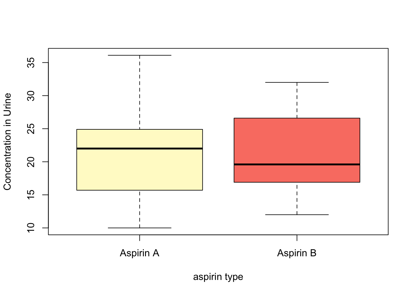
4.1 Determine the (approximate) sampling distribution for the difference in means
- ‘manual’ bootstrapping
- Since we want to take care of the natural pairing
of the data so for each patient,
- we will take difference between the aspirin A concentration levels and aspirin B concentration levels.
- Then we will perform a bootstrap on these computed differences.
B <- 10000
n <- dim(aspirinPharm)[1]
diffs <- aspirinPharm$Avals - aspirinPharm$Bvals
boot.diff <- replicate(10000,
                       {
                         x <- sample(diffs, size = n, replace = T)
                         mean(x)
                        }
)- Check the approximate sampling distribution for the mean (paired) differences.
hist(boot.diff, col = "lemonchiffon", freq = F,
     xlab = "sample mean difference",
     ylab = "probability",
     main = "Sample Mean Difference Distribution")
lines(density(boot.diff), col=6, lwd=3)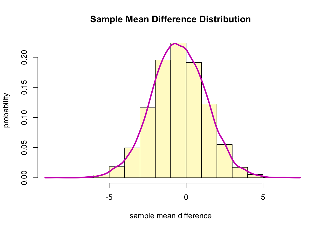
- The sampling distribution of the mean differences appears to be approximately normally distributed.
- When generating the sampling distribution, we need to be careful
because the two variables are measured on the same observational
unit and are not on two independent samples
- Bootstrap procedure needs to mimic the actual data collection process.
- However, paired data is not independent with each other.
- Thus, when we compare paired data such as this example, we compute the difference (or whatever value of interest) for each observation first.
- As a result, we will have one variable of interest. Then we can proceed with the bootstrap procedure as a single variable case.
4.2 Answer
- Question: is there a difference in the mean concentration level in the urine 1-hour after the aspirin was ingested between Aspirin A and B? (Use a 95% confidence interval)
- will use approximate sampling distribution
- The point estimate of the difference of the aspirin A and the
aspirin B is:
- Keep in mind that the point estimate is still computed based on the sample (NOT from the bootstrapped sampling distribution)
mean(aspirinPharm$Avals - aspirinPharm$Bvals) %>% round(1)## [1] -0.5- The 95% confidence interval is computed by using the
quantile()function from the bootstrapped sampling distribution.
(lb <- quantile(boot.diff, 0.025) %>% round(1))## 2.5%
## -3.9(ub <- quantile(boot.diff, 0.975) %>% round(1))## 97.5%
## 2.9- Conclusion: the 95% confidence interval is -3.9 to 2.9. Since the interval contains 0, there is no evidence that there is a difference in the mean concentration levels in urine 1-hour post ingestion of the aspirin.
4.3 Direct method: boot() and
boot.ci()
xbar.Diffs <- function(x, idx) {
    return(c(mean(x[idx]), var(x[idx])))
}

(diffs.bootObj <- boot(diffs, xbar.Diffs, 10000))
##
## ORDINARY NONPARAMETRIC BOOTSTRAP
##
##
## Call:
## boot(data = diffs, statistic = xbar.Diffs, R = 10000)
##
##
## Bootstrap Statistics :
## original bias std. error
## t1* -0.4680 0.0300408 1.76825
## t2* 81.6556 -3.5840770 23.71024# point estimate
diffs.bootObj$t0[1] %>% round(1)## [1] -0.5- The point estimate is [t1*, original], -0.5.
diffCI <- boot.ci(diffs.bootObj, conf = 0.95)

# Percentile method CI
diffCI$percent[4] %>% round(3)
## [1] -3.896diffCI$percent[5] %>% round(3)## [1] 2.996- Conclusion: the point estimate for the mean difference in concentration levels in the urine between aspirin A and aspirin B 1-hour post-ingestion is [t1*, original], -0.5 (from the original data, not from the bootstrapped sampling distribution). The corresponding 95% confidence interval is -3.896 to 2.996.
5. Bootstrap hypothesis testing
- Bootstrap hypothesis testing is relatively undeveloped, and is generally not used as much as another approach we will learn later(permutation test).
- However, there are some ways to do bootstrap tests.
- <1> One general approximate approach is to base a test on a
bootstrap confidence interval
- To reject the \(H_0\) null hypothesis if the interval fails to inlcude \(\theta_0\).
- <2> Anoother general approach is to sample in a way that is
consistent with the null hypothesis, then calculate a \(p\)-value as a tail probability like we do
in permutation tests.
- One naive way to do this is to modify the observations, e.g. to subtract the difference between the observed statistical value from the sample (\(\hat{\theta}\)) and the null hypothesis value for the parameter (\(\theta_0\)) each observation.
- In other words, in the original sample, we would substract the value \(\hat{\theta}-\theta_0\) from each observation and then do the bootstrap on these modified values.
- However, this is not highly recommended because
- it is not accurate for skewed populations,
- it can give impossible data (e.g. negative time measurements), and
- it does not generalize well to other applications such as relative risk, correlation, regression, or categorical data.
- <1> One general approximate approach is to base a test on a
bootstrap confidence interval
- We will just base a test on a bootstrap confidence interval to reject the null hypothesis.
- Specifically, if the significance level is \(\alpha\), we would use a \((1-\alpha) \times 100\)% confidence interval to determine whether we would reject the null hypothesis or not.